Theory and Applications of Boosting
Rob Schapire
« Theory and Applications of Boosting
Robert Schapire
Boosting is a general method for producing a very accurate classification rule by combining rough and moderately inaccurate “rules of thumb.” While rooted in a theoretical framework of machine learning, boosting has been found to perform quite well empirically. This tutorial will focus on the boosting algorithm AdaBoost, and will explain the underlying theory of boosting, including explanations that have been given as to why boosting often does not suffer from overfitting, as well as interpretations based on game theory, optimization, statistics, and maximum entropy. Some practical applications and extensions of boosting will also be described.
Scroll with j/k | | | Size
1
![Slide: Example: How May I Help You?
[Gorin et al.]
goal: automatically categorize type of call requested by phone customer (Collect, CallingCard, PersonToPerson, etc.) yes Id like to place a collect call long distance please (Collect) operator I need to make a call but I need to bill it to my office (ThirdNumber) yes Id like to place a call on my master card please (CallingCard) I just called a number in sioux city and I musta rang the wrong number because I got the wrong party and I would like to have that taken off of my bill (BillingCredit) observation:
easy to nd rules of thumb that are often correct e.g.: IF card occurs in utterance THEN predict CallingCard hard to nd single highly accurate prediction rule](https://yosinski.com/mlss12/media/slides/MLSS-2012-Schapire-Theory-and-Applications-of-Boosting_002.png)
Example: How May I Help You?
[Gorin et al.]
goal: automatically categorize type of call requested by phone customer (Collect, CallingCard, PersonToPerson, etc.) yes Id like to place a collect call long distance please (Collect) operator I need to make a call but I need to bill it to my office (ThirdNumber) yes Id like to place a call on my master card please (CallingCard) I just called a number in sioux city and I musta rang the wrong number because I got the wrong party and I would like to have that taken off of my bill (BillingCredit) observation:
easy to nd rules of thumb that are often correct e.g.: IF card occurs in utterance THEN predict CallingCard hard to nd single highly accurate prediction rule
2
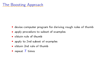
The Boosting Approach
devise computer program for deriving rough rules of thumb apply procedure to subset of examples obtain rule of thumb apply to 2nd subset of examples obtain 2nd rule of thumb repeat T times
3
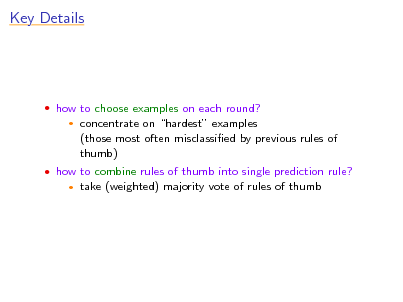
Key Details
how to choose examples on each round?
concentrate on hardest examples (those most often misclassied by previous rules of thumb) take (weighted) majority vote of rules of thumb
how to combine rules of thumb into single prediction rule?
4
![Slide: Boosting
boosting = general method of converting rough rules of
thumb into highly accurate prediction rule
technically:
assume given weak learning algorithm that can consistently nd classiers (rules of thumb) at least slightly better than random, say, accuracy 55% (in two-class setting) [ weak learning assumption ] given sucient data, a boosting algorithm can provably construct single classier with very high accuracy, say, 99%](https://yosinski.com/mlss12/media/slides/MLSS-2012-Schapire-Theory-and-Applications-of-Boosting_005.png)
Boosting
boosting = general method of converting rough rules of
thumb into highly accurate prediction rule
technically:
assume given weak learning algorithm that can consistently nd classiers (rules of thumb) at least slightly better than random, say, accuracy 55% (in two-class setting) [ weak learning assumption ] given sucient data, a boosting algorithm can provably construct single classier with very high accuracy, say, 99%
5
Outline of Tutorial
basic algorithm and core theory fundamental perspectives practical extensions advanced topics
6

Preamble: Early History
7
![Slide: Strong and Weak Learnability
boostings roots are in PAC learning model strong PAC learning algorithm:
[Valiant 84]
get random examples from unknown, arbitrary distribution
for any distribution with high probability given polynomially many examples (and polynomial time) can nd classier with arbitrarily small generalization error same, but generalization error only needs to be slightly better than random guessing ( 1 ) 2 does weak learnability imply strong learnability?
weak PAC learning algorithm
[Kearns & Valiant 88]:](https://yosinski.com/mlss12/media/slides/MLSS-2012-Schapire-Theory-and-Applications-of-Boosting_008.png)
Strong and Weak Learnability
boostings roots are in PAC learning model strong PAC learning algorithm:
[Valiant 84]
get random examples from unknown, arbitrary distribution
for any distribution with high probability given polynomially many examples (and polynomial time) can nd classier with arbitrarily small generalization error same, but generalization error only needs to be slightly better than random guessing ( 1 ) 2 does weak learnability imply strong learnability?
weak PAC learning algorithm
[Kearns & Valiant 88]:
8
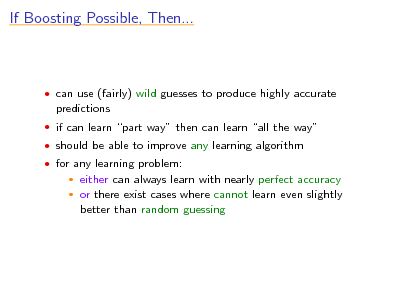
If Boosting Possible, Then...
can use (fairly) wild guesses to produce highly accurate
predictions
if can learn part way then can learn all the way should be able to improve any learning algorithm for any learning problem:
either can always learn with nearly perfect accuracy or there exist cases where cannot learn even slightly better than random guessing
9
![Slide: First Boosting Algorithms
[Schapire 89]:
rst provable boosting algorithm optimal algorithm that boosts by majority rst experiments using boosting limited by practical drawbacks introduced AdaBoost algorithm strong practical advantages over previous boosting algorithms
[Freund 90]:
[Drucker, Schapire & Simard 92]:
[Freund & Schapire 95]:](https://yosinski.com/mlss12/media/slides/MLSS-2012-Schapire-Theory-and-Applications-of-Boosting_010.png)
First Boosting Algorithms
[Schapire 89]:
rst provable boosting algorithm optimal algorithm that boosts by majority rst experiments using boosting limited by practical drawbacks introduced AdaBoost algorithm strong practical advantages over previous boosting algorithms
[Freund 90]:
[Drucker, Schapire & Simard 92]:
[Freund & Schapire 95]:
10
Basic Algorithm and Core Theory
introduction to AdaBoost analysis of training error analysis of test error
and the margins theory
experiments and applications
11
Basic Algorithm and Core Theory
introduction to AdaBoost analysis of training error analysis of test error
and the margins theory
experiments and applications
12
![Slide: A Formal Description of Boosting
given training set for t = 1, . . . , T :
(x1 , y1 ), . . . , (xm , ym )
yi {1, +1} correct label of instance xi X
construct distribution Dt on {1, . . . , m} nd weak classier (rule of thumb) ht : X {1, +1} with error t on Dt : t = PriDt [ht (xi ) = yi ]
output nal/combined classier Hnal](https://yosinski.com/mlss12/media/slides/MLSS-2012-Schapire-Theory-and-Applications-of-Boosting_013.png)
A Formal Description of Boosting
given training set for t = 1, . . . , T :
(x1 , y1 ), . . . , (xm , ym )
yi {1, +1} correct label of instance xi X
construct distribution Dt on {1, . . . , m} nd weak classier (rule of thumb) ht : X {1, +1} with error t on Dt : t = PriDt [ht (xi ) = yi ]
output nal/combined classier Hnal
13
![Slide: AdaBoost
constructing Dt :
[with Freund]
D1 (i) = 1/m given Dt and ht : Dt+1 (i) = = Dt (i) e t if yi = ht (xi ) if yi = ht (xi ) e t Zt Dt (i) exp(t yi ht (xi )) Zt
where Zt = normalization factor 1 1 t >0 t = ln 2 t nal classier:
Hnal (x) = sign
t
t ht (x)](https://yosinski.com/mlss12/media/slides/MLSS-2012-Schapire-Theory-and-Applications-of-Boosting_014.png)
AdaBoost
constructing Dt :
[with Freund]
D1 (i) = 1/m given Dt and ht : Dt+1 (i) = = Dt (i) e t if yi = ht (xi ) if yi = ht (xi ) e t Zt Dt (i) exp(t yi ht (xi )) Zt
where Zt = normalization factor 1 1 t >0 t = ln 2 t nal classier:
Hnal (x) = sign
t
t ht (x)
14
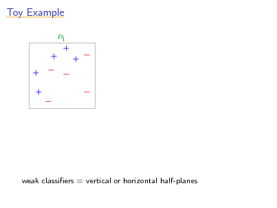
Toy Example
D1
weak classiers = vertical or horizontal half-planes
15
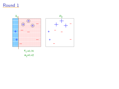
Round 1
1 11111 1111111111111 00000 0000000000000 11111 1111111111111 00000 0000000000000 11111 1111111111111 00000 0000000000000 11111 1111111111111 00000 0000000000000 11111 1111111111111 00000 0000000000000 11111 1111111111111 00000 0000000000000 11111 1111111111111 00000 0000000000000 11111 00000 1111111111111 0000000000000 11111 00000 1111111111111 0000000000000 11111 1111111111111 00000 0000000000000 11111 1111111111111 00000 0000000000000 11111 00000 1111111111111 0000000000000 11111 00000 1111111111111 0000000000000 11111 1111111111111 00000 0000000000000 11111 1111111111111 00000 0000000000000 11111 00000 1111111111111 0000000000000 11111 00000 1111111111111 0000000000000 11111 1111111111111 00000 0000000000000 11111 1111111111111 00000 0000000000000 11111 00000 1111111111111 0000000000000 11111 00000 1111111111111 0000000000000 11111 1111111111111 00000 0000000000000 11111 1111111111111 00000 0000000000000 11111 00000 1111111111111 0000000000000 11111 00000 1111111111111 0000000000000 11111 00000 1111111111111 0000000000000 11111 1111111111111 00000 0000000000000 11111 1111111111111 00000 0000000000000 11111 00000 1111111111111 0000000000000 11111 00000 1111111111111 0000000000000 11111 1111111111111 00000 0000000000000 1 =0.30 1=0.42 h D2
16
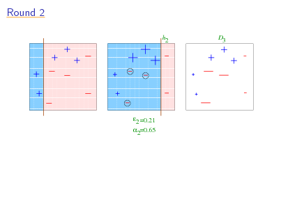
Round 2
11111 1111111111111 00000 0000000000000 11111 1111111111111 00000 0000000000000 11111 1111111111111 00000 0000000000000 11111 1111111111111 00000 0000000000000 11111 1111111111111 00000 0000000000000 11111 1111111111111 00000 0000000000000 11111 1111111111111 00000 0000000000000 11111 00000 1111111111111 0000000000000 11111 00000 1111111111111 0000000000000 11111 1111111111111 00000 0000000000000 11111 1111111111111 00000 0000000000000 11111 00000 1111111111111 0000000000000 11111 00000 1111111111111 0000000000000 11111 1111111111111 00000 0000000000000 11111 1111111111111 00000 0000000000000 11111 00000 1111111111111 0000000000000 11111 00000 1111111111111 0000000000000 11111 1111111111111 00000 0000000000000 11111 1111111111111 00000 0000000000000 11111 00000 1111111111111 0000000000000 11111 00000 1111111111111 0000000000000 11111 1111111111111 00000 0000000000000 11111 1111111111111 00000 0000000000000 11111 00000 1111111111111 0000000000000 11111 00000 1111111111111 0000000000000 11111 00000 1111111111111 0000000000000 11111 1111111111111 00000 0000000000000 11111 1111111111111 00000 0000000000000 11111 00000 1111111111111 0000000000000 11111 00000 1111111111111 0000000000000 11111 1111111111111 00000 0000000000000 1111111111111 2 00000000000001111 11111111111110000 1111 00000000000000000 11111111111111111 00000000000000000 11111111111111111 00000000000000000 11111111111111111 00000000000000000 11111111111111111 00000000000000000 11111111111111111 00000000000000000 11111111111111111 00000000000000000 11111111111111111 00000000000000000 11111111111111111 00000000000000000 11111111111111111 00000000000000000 11111111111111111 00000000000000000 11111111111111111 00000000000000000 11111111111111111 00000000000000000 11111111111111111 00000000000000000 11111111111111111 00000000000000000 11111111111111111 00000000000000000 11111111111111111 00000000000000000 11111111111111111 00000000000000000 11111111111111111 00000000000000000 11111111111111111 00000000000000000 11111111111111111 00000000000000000 11111111111111111 00000000000000000 11111111111111111 00000000000000000 11111111111111111 00000000000000000 11111111111111111 00000000000000000 11111111111111111 00000000000001111 11111111111110000 00000000000000000 11111111111111111 00000000000000000 11111111111111111 00000000000000000 11111111111111111 00000000000000000
h
D3
2 =0.21 2=0.65
17
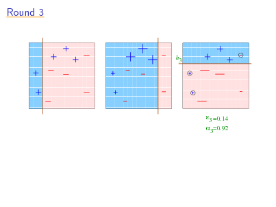
Round 3
11111 1111111111111 00000 0000000000000 11111 1111111111111 00000 0000000000000 11111 1111111111111 00000 0000000000000 11111 1111111111111 00000 0000000000000 11111 1111111111111 00000 0000000000000 11111 1111111111111 00000 0000000000000 11111 1111111111111 00000 0000000000000 11111 00000 1111111111111 0000000000000 11111 00000 1111111111111 0000000000000 11111 1111111111111 00000 0000000000000 11111 1111111111111 00000 0000000000000 11111 00000 1111111111111 0000000000000 11111 00000 1111111111111 0000000000000 11111 1111111111111 00000 0000000000000 11111 1111111111111 00000 0000000000000 11111 00000 1111111111111 0000000000000 11111 00000 1111111111111 0000000000000 11111 1111111111111 00000 0000000000000 11111 1111111111111 00000 0000000000000 11111 00000 1111111111111 0000000000000 11111 00000 1111111111111 0000000000000 11111 1111111111111 00000 0000000000000 11111 1111111111111 00000 0000000000000 11111 00000 1111111111111 0000000000000 11111 00000 1111111111111 0000000000000 11111 00000 1111111111111 0000000000000 11111 1111111111111 00000 0000000000000 11111 1111111111111 00000 0000000000000 11111 00000 1111111111111 0000000000000 11111 00000 1111111111111 0000000000000 11111 1111111111111 00000 0000000000000 1111111111111 00000000000001111 111111111111111 000000000000000 11111111111110000 1111 00000000000000000 111111111111111 000000000000000 11111111111111111 00000000000000000 111111111111111 000000000000000 11111111111111111 000000000000000 00000000000000000 111111111111111 11111111111111111 111111111111111 000000000000000 00000000000000000 11111111111111111 111111111111111 000000000000000 00000000000000000 11111111111111111 111111111111111 00000000000000000 11111111111111111 00000000000000000 h 000000000000000 111111111111111 000000000000000 000000000000000 11111111111111111 00000000000000000 111111111111111 11111111111111111 111111111111111 00000000000000000 3 000000000000000 11111111111111111 00000000000000000 111111111111111 000000000000000 11111111111111111 00000000000000000 000000000000000 111111111111111 11111111111111111 00000000000000000 000000000000000 111111111111111 11111111111111111 00000000000000000 000000000000000 111111111111111 11111111111111111 00000000000000000 111111111111111 000000000000000 11111111111111111 00000000000000000 000000000000000 111111111111111 11111111111111111 00000000000000000 000000000000000 111111111111111 11111111111111111 00000000000000000 000000000000000 111111111111111 11111111111111111 00000000000000000 111111111111111 000000000000000 11111111111111111 00000000000000000 000000000000000 111111111111111 11111111111111111 00000000000000000 000000000000000 111111111111111 11111111111111111 00000000000000000 000000000000000 111111111111111 11111111111111111 00000000000000000 111111111111111 000000000000000 11111111111111111 00000000000000000 000000000000000 111111111111111 11111111111111111 00000000000000000 000000000000000 111111111111111 11111111111111111 00000000000000000 000000000000000 111111111111111 11111111111111111 00000000000000000 000000000000000 111111111111111 11111111111111111 00000000000000000 111111111111111 000000000000000 11111111111111111 00000000000000000 000000000000000 111111111111111 11111111111111111 00000000000000000 000000000000000 111111111111111 11111111111111111 00000000000000000 000000000000000 111111111111111
3 =0.14 3=0.92
18
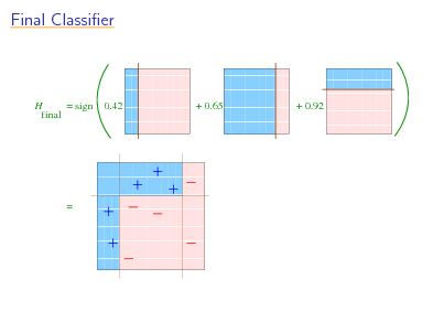
Final Classier
000 000000000 111 111111111 000 000000000 111 111111111 111 000 111111111 000000000 000 000000000 111 111111111 000 000000000 111 111111111 000 000000000 111 111111111 111 000 111111111 000000000 000 000000000 111 111111111 000 000000000 111 111111111 000 000000000 111 111 000 111111111 000000000 0.42 111111111 + 000 000000000 111 111111111 000 000000000 111 111111111 000 000000000 111 111111111 000 000000000 111 111111111 111 000 111111111 000000000 000 000000000 111 111111111 000 000000000 111 111111111 000 000000000 111 111111111 000000000 00 111111111 11 000000000 00 111111111 11 111111111 000000000 11 00 000000000 00 111111111 11 000000000 00 111111111 11 000000000 00 111111111 11 111111111 000000000 11 00 000000000 00 111111111 11 000000000 00 111111111 11 000000000 00 111111111 11 111111111 000000000 11 00 0.65 000000000 00 111111111 11 000000000 00 111111111 11 000000000 00 111111111 11 000000000 00 111111111 11 111111111 000000000 11 00 000000000 00 111111111 11 000000000 00 111111111 11 000000000 00 111111111 11 1111111111 0000000000 1111111111 0000000000 1111111111 0000000000 1111111111 0000000000 1111111111 0000000000 1111111111 0000000000 1111111111 0000000000 1111111111 0000000000 0000000000 1111111111 1111111111 0000000000 1111111111 0000000000 1111111111 0000000000 0000000000 1111111111 1111111111 0000000000 1111111111 0000000000 1111111111 0000000000 1111111111 0000000000 0000000000 1111111111 1111111111 0000000000 1111111111 0000000000
H = sign final
+ 0.92
=
1111111111111 0000000000000 11111 00000 111111111111 000000000000 1111111111111 0000000000000 11111 00000 111111111111 000000000000 1111111111111 0000000000000 11111 00000 111111111111 000000000000 0000000000000 1111111111111 11111 00000 111111111111 000000000000 0000000000000 1111111111111 11111 111111111111 00000 000000000000 1111111111111 0000000000000 11111 00000 111111111111 000000000000 1111111111111 0000000000000 11111 111111111111 00000 000000000000 1111111111111 0000000000000 11111 00000 111111111111 000000000000 1111111111111 0000000000000 11111 111111111111 00000 000000000000 0000000000000 1111111111111 11111 111111111111 00000 000000000000 1111111111111 0000000000000 11111 00000 111111111111 000000000000 11111 111111111111 00000 000000000000 11111 00000 111111111111 000000000000 11111 00000 111111111111 000000000000 11111 111111111111 00000 000000000000 11111 00000 111111111111 000000000000 11111 111111111111 00000 000000000000 11111 111111111111 00000 000000000000 11111 00000 111111111111 000000000000 11111 111111111111 00000 000000000000 11111 00000 111111111111 000000000000 11111 00000 111111111111 000000000000 11111 111111111111 00000 000000000000 11111 00000 111111111111 000000000000 11111 111111111111 00000 000000000000 11111 111111111111 00000 000000000000 11111 00000 111111111111 000000000000 11111 00000 111111111111 000000000000 11111 00000 111111111111 000000000000 11111 111111111111 00000 000000000000 11111 111111111111 00000 000000000000 11111 00000 111111111111 000000000000
19
Basic Algorithm and Core Theory
introduction to AdaBoost analysis of training error analysis of test error
and the margins theory
experiments and applications
20
![Slide: Analyzing the Training Error
Theorem:
[with Freund]
write t as then
1 2
t
[ t = edge ] 2 t (1 t )
t 2 1 4t t
training error(Hnal ) =
exp 2
t
2 t
so: if t : t > 0
then training error(Hnal ) e 2 T AdaBoost is adaptive: does not need to know or T a priori can exploit t
2](https://yosinski.com/mlss12/media/slides/MLSS-2012-Schapire-Theory-and-Applications-of-Boosting_021.png)
Analyzing the Training Error
Theorem:
[with Freund]
write t as then
1 2
t
[ t = edge ] 2 t (1 t )
t 2 1 4t t
training error(Hnal ) =
exp 2
t
2 t
so: if t : t > 0
then training error(Hnal ) e 2 T AdaBoost is adaptive: does not need to know or T a priori can exploit t
2
21
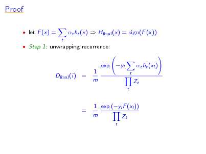
Proof
let F (x) =
t
t ht (x) Hnal (x) = sign(F (x))
Step 1: unwrapping recurrence:
Dnal (i) =
1 m
exp yi
t
t ht (xi ) Zt
t
=
1 exp (yi F (xi )) m Zt
t
22
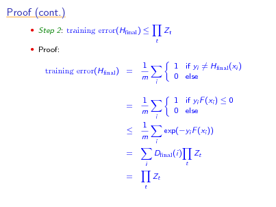
Proof (cont.)
Step 2: training error(Hnal )
t
Zt
Proof:
training error(Hnal ) =
1 m 1 m 1 m
i
1 if yi = Hnal (xi ) 0 else 1 if yi F (xi ) 0 0 else exp(yi F (xi ))
= =
i
i
Dnal (i)
i t
Zt
=
t
Zt
23
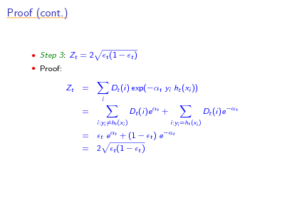
Proof (cont.)
Step 3: Zt = 2 Proof:
t (1 t )
Zt
=
i
Dt (i) exp(t yi ht (xi )) Dt (i)e t +
i:yi =ht (xi ) t e t + (1
= =
Dt (i)e t
t ) e
i:yi =ht (xi ) t
= 2 t (1 t )
24
Basic Algorithm and Core Theory
introduction to AdaBoost analysis of training error analysis of test error
and the margins theory
experiments and applications
25
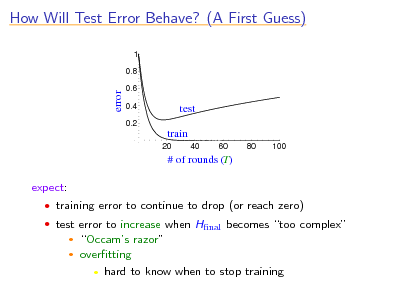
How Will Test Error Behave? (A First Guess)
1 0.8
error
0.6 0.4 0.2
test train
20 40 60 80 100
# of rounds (T)
expect:
training error to continue to drop (or reach zero) test error to increase when Hnal becomes too complex
Occams razor overtting hard to know when to stop training
26
![Slide: Technically...
with high probability:
generalization error training error + O bound depends on m = # training examples d = complexity of weak classiers T = # rounds
dT m
generalization error = E [test error] predicts overtting](https://yosinski.com/mlss12/media/slides/MLSS-2012-Schapire-Theory-and-Applications-of-Boosting_027.png)
Technically...
with high probability:
generalization error training error + O bound depends on m = # training examples d = complexity of weak classiers T = # rounds
dT m
generalization error = E [test error] predicts overtting
27
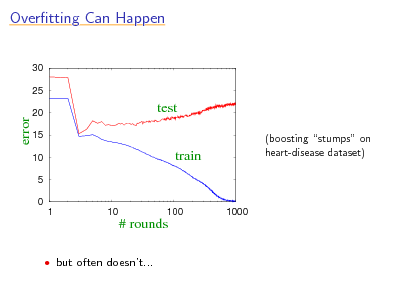
Overtting Can Happen
30 25
error
20 15 10 5 0 1 10
test train
(boosting stumps on heart-disease dataset)
100
1000
# rounds
but often doesnt...
28
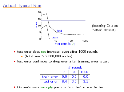
Actual Typical Run
20 15
error
10 5 0
test train
10 100 1000
(boosting C4.5 on letter dataset)
# of rounds (T)
test error does not increase, even after 1000 rounds
(total size > 2,000,000 nodes) test error continues to drop even after training error is zero!
train error test error
# rounds 5 100 1000 0.0 0.0 0.0 8.4 3.3 3.1
Occams razor wrongly predicts simpler rule is better
29
![Slide: A Better Story: The Margins Explanation
key idea:
[with Freund, Bartlett & Lee]
training error only measures whether classications are right or wrong should also consider condence of classications
recall: Hnal is weighted majority vote of weak classiers measure condence by margin = strength of the vote
= (weighted fraction voting correctly) (weighted fraction voting incorrectly)
high conf. incorrect 1 Hfinal incorrect high conf. correct Hfinal correct +1
low conf. 0](https://yosinski.com/mlss12/media/slides/MLSS-2012-Schapire-Theory-and-Applications-of-Boosting_030.png)
A Better Story: The Margins Explanation
key idea:
[with Freund, Bartlett & Lee]
training error only measures whether classications are right or wrong should also consider condence of classications
recall: Hnal is weighted majority vote of weak classiers measure condence by margin = strength of the vote
= (weighted fraction voting correctly) (weighted fraction voting incorrectly)
high conf. incorrect 1 Hfinal incorrect high conf. correct Hfinal correct +1
low conf. 0
30
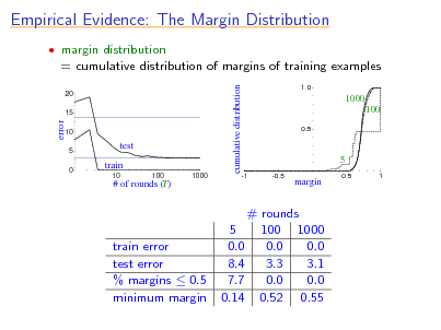
Empirical Evidence: The Margin Distribution
margin distribution
= cumulative distribution of margins of training examples
cumulative distribution
20 15
1.0
1000 100
0.5
error
10 5 0
test train
10 100 1000
5
-1 -0.5
# of rounds (T)
margin
0.5
1
train error test error % margins 0.5 minimum margin
# rounds 5 100 1000 0.0 0.0 0.0 8.4 3.3 3.1 7.7 0.0 0.0 0.14 0.52 0.55
31
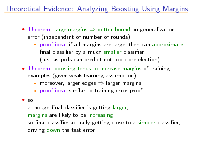
Theoretical Evidence: Analyzing Boosting Using Margins
Theorem: large margins better bound on generalization
error (independent of number of rounds) proof idea: if all margins are large, then can approximate nal classier by a much smaller classier (just as polls can predict not-too-close election)
Theorem: boosting tends to increase margins of training
examples (given weak learning assumption) moreover, larger edges larger margins proof idea: similar to training error proof
so:
although nal classier is getting larger, margins are likely to be increasing, so nal classier actually getting close to a simpler classier, driving down the test error
32
![Slide: More Technically...
with high probability, > 0 :
generalization error Pr[margin ] + O
d/m
(Pr[ ] = empirical probability)
bound depends on m = # training examples d = complexity of weak classiers entire distribution of margins of training examples
1 2
Pr[margin ] 0 exponentially fast (in T ) if t <
(t)
so: if weak learning assumption holds, then all examples will quickly have large margins](https://yosinski.com/mlss12/media/slides/MLSS-2012-Schapire-Theory-and-Applications-of-Boosting_033.png)
More Technically...
with high probability, > 0 :
generalization error Pr[margin ] + O
d/m
(Pr[ ] = empirical probability)
bound depends on m = # training examples d = complexity of weak classiers entire distribution of margins of training examples
1 2
Pr[margin ] 0 exponentially fast (in T ) if t <
(t)
so: if weak learning assumption holds, then all examples will quickly have large margins
33
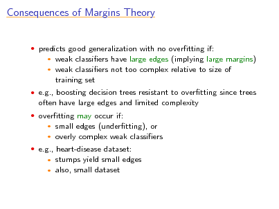
Consequences of Margins Theory
predicts good generalization with no overtting if:
weak classiers have large edges (implying large margins) weak classiers not too complex relative to size of training set
e.g., boosting decision trees resistant to overtting since trees
often have large edges and limited complexity
overtting may occur if:
small edges (undertting), or overly complex weak classiers
e.g., heart-disease dataset:
stumps yield small edges also, small dataset
34
![Slide: Improved Boosting with Better Margin-Maximization?
can design algorithms more eective than AdaBoost at
maximizing the minimum margin
in practice, often perform worse why?? more aggressive margin maximization seems to lead to: [Breiman]
more complex weak classiers (even using same weak learner); or higher minimum margins, but margin distributions that are lower overall
[with Reyzin]](https://yosinski.com/mlss12/media/slides/MLSS-2012-Schapire-Theory-and-Applications-of-Boosting_035.png)
Improved Boosting with Better Margin-Maximization?
can design algorithms more eective than AdaBoost at
maximizing the minimum margin
in practice, often perform worse why?? more aggressive margin maximization seems to lead to: [Breiman]
more complex weak classiers (even using same weak learner); or higher minimum margins, but margin distributions that are lower overall
[with Reyzin]
35
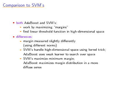
Comparison to SVMs
both AdaBoost and SVMs:
work by maximizing margins nd linear threshold function in high-dimensional space
dierences:
margin measured slightly dierently (using dierent norms) SVMs handle high-dimensional space using kernel trick; AdaBoost uses weak learner to search over space SVMs maximize minimum margin; AdaBoost maximizes margin distribution in a more diuse sense
36
Basic Algorithm and Core Theory
introduction to AdaBoost analysis of training error analysis of test error
and the margins theory
experiments and applications
37
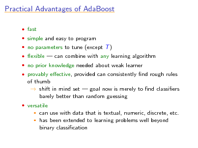
Practical Advantages of AdaBoost
fast simple and easy to program no parameters to tune (except T ) exible can combine with any learning algorithm no prior knowledge needed about weak learner provably eective, provided can consistently nd rough rules
of thumb shift in mind set goal now is merely to nd classiers barely better than random guessing
versatile
can use with data that is textual, numeric, discrete, etc. has been extended to learning problems well beyond binary classication
38
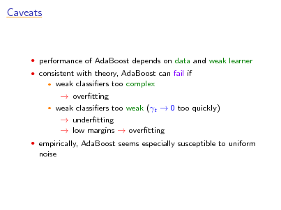
Caveats
performance of AdaBoost depends on data and weak learner consistent with theory, AdaBoost can fail if
weak classiers too complex overtting weak classiers too weak (t 0 too quickly) undertting low margins overtting
empirically, AdaBoost seems especially susceptible to uniform
noise
39
![Slide: UCI Experiments
tested AdaBoost on UCI benchmarks used:
[with Freund]
C4.5 (Quinlans decision tree algorithm) decision stumps: very simple rules of thumb that test on single attributes
eye color = brown ? yes predict +1 no predict -1
height > 5 feet ? yes predict -1 no predict +1](https://yosinski.com/mlss12/media/slides/MLSS-2012-Schapire-Theory-and-Applications-of-Boosting_040.png)
UCI Experiments
tested AdaBoost on UCI benchmarks used:
[with Freund]
C4.5 (Quinlans decision tree algorithm) decision stumps: very simple rules of thumb that test on single attributes
eye color = brown ? yes predict +1 no predict -1
height > 5 feet ? yes predict -1 no predict +1
40
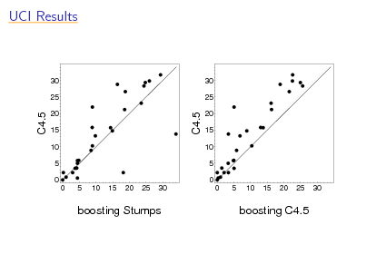
UCI Results
30 25
30 25
C4.5
C4.5
20 15 10 5 0 0 5 10 15 20 25 30
20 15 10 5 0 0 5 10 15 20 25 30
boosting Stumps
boosting C4.5
41
![Slide: Application: Detecting Faces
[Viola & Jones]
problem: nd faces in photograph or movie weak classiers: detect light/dark rectangles in image
many clever tricks to make extremely fast and accurate](https://yosinski.com/mlss12/media/slides/MLSS-2012-Schapire-Theory-and-Applications-of-Boosting_042.png)
Application: Detecting Faces
[Viola & Jones]
problem: nd faces in photograph or movie weak classiers: detect light/dark rectangles in image
many clever tricks to make extremely fast and accurate
42
![Slide: Application: Human-Computer Spoken Dialogue
[with Rahim, Di Fabbrizio, Dutton, Gupta, Hollister & Riccardi]
application: automatic store front or help desk for AT&T
Labs Natural Voices business
caller can request demo, pricing information, technical
support, sales agent, etc.
interactive dialogue](https://yosinski.com/mlss12/media/slides/MLSS-2012-Schapire-Theory-and-Applications-of-Boosting_043.png)
Application: Human-Computer Spoken Dialogue
[with Rahim, Di Fabbrizio, Dutton, Gupta, Hollister & Riccardi]
application: automatic store front or help desk for AT&T
Labs Natural Voices business
caller can request demo, pricing information, technical
support, sales agent, etc.
interactive dialogue
43
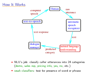
How It Works
computer speech texttospeech Human raw utterance
automatic speech recognizer text
text response
dialogue manager
predicted category
natural language understanding
NLUs job: classify caller utterances into 24 categories
(demo, sales rep, pricing info, yes, no, etc.)
weak classiers: test for presence of word or phrase
44
Problem: Labels are Expensive
for spoken-dialogue task
getting examples is cheap getting labels is expensive must be annotated by humans
how to reduce number of labels needed?
45
![Slide: Active Learning
[with Tur & Hakkani-Tr] u
idea:
use selective sampling to choose which examples to label focus on least condent examples [Lewis & Gale]
for boosting, use (absolute) margin as natural condence measure [Abe & Mamitsuka]](https://yosinski.com/mlss12/media/slides/MLSS-2012-Schapire-Theory-and-Applications-of-Boosting_046.png)
Active Learning
[with Tur & Hakkani-Tr] u
idea:
use selective sampling to choose which examples to label focus on least condent examples [Lewis & Gale]
for boosting, use (absolute) margin as natural condence measure [Abe & Mamitsuka]
46
Labeling Scheme
start with pool of unlabeled examples choose (say) 500 examples at random for labeling run boosting on all labeled examples
get combined classier F choose examples with minimum |F (x)| (proportional to absolute margin)
pick (say) 250 additional examples from pool for labeling
repeat
47
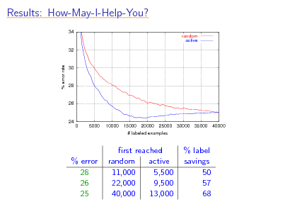
Results: How-May-I-Help-You?
34 random active
32
% error rate
30
28
26
24 0 5000 10000 15000 20000 25000 # labeled examples 30000 35000 40000
% error 28 26 25
rst reached random active 11,000 5,500 22,000 9,500 40,000 13,000
% label savings 50 57 68
48
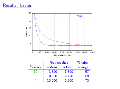
Results: Letter
25 random active
20
% error rate
15
10
5
0 0 2000 4000 6000 8000 10000 # labeled examples 12000 14000 16000
% error 10 5 4
rst reached random active 3,500 1,500 9,000 2,750 13,000 3,500
% label savings 57 69 73
49
Fundamental Perspectives
game theory loss minimization an information-geometric view
50
Fundamental Perspectives
game theory loss minimization an information-geometric view
51
![Slide: Just a Game
[with Freund]
can view boosting as a game, a formal interaction between
booster and weak learner
on each round t:
booster chooses distribution Dt weak learner responds with weak classier ht
game theory: studies interactions between all sorts of
players](https://yosinski.com/mlss12/media/slides/MLSS-2012-Schapire-Theory-and-Applications-of-Boosting_052.png)
Just a Game
[with Freund]
can view boosting as a game, a formal interaction between
booster and weak learner
on each round t:
booster chooses distribution Dt weak learner responds with weak classier ht
game theory: studies interactions between all sorts of
players
52
![Slide: Games
game dened by matrix M:
Rock Paper Scissors
Rock 1/2 0 1
Paper 1 1/2 0
Scissors 0 1 1/2
row player (Mindy) chooses row i column player (Max) chooses column j (simultaneously) Mindys goal: minimize her loss M(i, j) assume (wlog) all entries in [0, 1]](https://yosinski.com/mlss12/media/slides/MLSS-2012-Schapire-Theory-and-Applications-of-Boosting_053.png)
Games
game dened by matrix M:
Rock Paper Scissors
Rock 1/2 0 1
Paper 1 1/2 0
Scissors 0 1 1/2
row player (Mindy) chooses row i column player (Max) chooses column j (simultaneously) Mindys goal: minimize her loss M(i, j) assume (wlog) all entries in [0, 1]
53
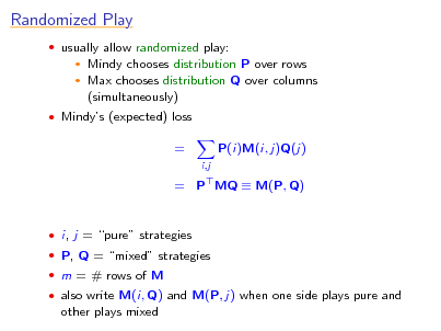
Randomized Play
usually allow randomized play:
Mindy chooses distribution P over rows Max chooses distribution Q over columns (simultaneously)
Mindys (expected) loss
=
i,j
P(i)M(i, j)Q(j)
= P MQ M(P, Q)
i, j = pure strategies P, Q = mixed strategies m = # rows of M also write M(i, Q) and M(P, j) when one side plays pure and
other plays mixed
54
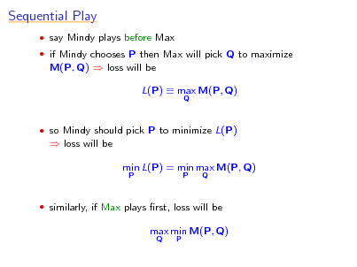
Sequential Play
say Mindy plays before Max if Mindy chooses P then Max will pick Q to maximize
M(P, Q) loss will be L(P) max M(P, Q)
Q
so Mindy should pick P to minimize L(P)
loss will be min L(P) = min max M(P, Q)
P P Q
similarly, if Max plays rst, loss will be
max min M(P, Q)
Q P
55
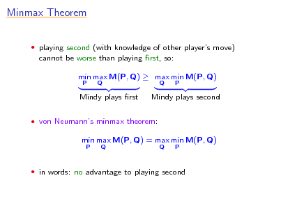
Minmax Theorem
playing second (with knowledge of other players move)
cannot be worse than playing rst, so: min max M(P, Q) max min M(P, Q)
P Q Q P
Mindy plays rst
Mindy plays second
von Neumanns minmax theorem:
min max M(P, Q) = max min M(P, Q)
P Q Q P
in words: no advantage to playing second
56
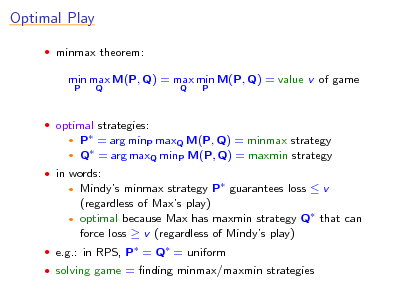
Optimal Play
minmax theorem:
min max M(P, Q) = max min M(P, Q) = value v of game
P Q Q P
optimal strategies:
P = arg minP maxQ M(P, Q) = minmax strategy Q = arg maxQ minP M(P, Q) = maxmin strategy
in words:
Mindys minmax strategy P guarantees loss v (regardless of Maxs play) optimal because Max has maxmin strategy Q that can force loss v (regardless of Mindys play)
e.g.: in RPS, P = Q = uniform solving game = nding minmax/maxmin strategies
57
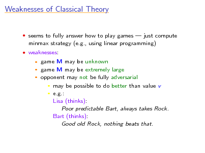
Weaknesses of Classical Theory
seems to fully answer how to play games just compute
minmax strategy (e.g., using linear programming)
weaknesses:
game M may be unknown game M may be extremely large opponent may not be fully adversarial may be possible to do better than value v e.g.: Lisa (thinks): Poor predictable Bart, always takes Rock. Bart (thinks): Good old Rock, nothing beats that.
58
Repeated Play
if only playing once, hopeless to overcome ignorance of game
M or opponent
but if game played repeatedly, may be possible to learn to
play well
goal: play (almost) as well as if knew game and how
opponent would play ahead of time
59
![Slide: Repeated Play (cont.)
M unknown for t = 1, . . . , T :
Mindy chooses Pt Max chooses Qt (possibly depending on Pt ) Mindys loss = M(Pt , Qt ) Mindy observes loss M(i, Qt ) of each pure strategy i
want:
1 T
T
M(Pt , Qt ) min
t=1 P
1 T
T
M(P, Qt ) + [small amount]
t=1
actual average loss
best loss (in hindsight)](https://yosinski.com/mlss12/media/slides/MLSS-2012-Schapire-Theory-and-Applications-of-Boosting_060.png)
Repeated Play (cont.)
M unknown for t = 1, . . . , T :
Mindy chooses Pt Max chooses Qt (possibly depending on Pt ) Mindys loss = M(Pt , Qt ) Mindy observes loss M(i, Qt ) of each pure strategy i
want:
1 T
T
M(Pt , Qt ) min
t=1 P
1 T
T
M(P, Qt ) + [small amount]
t=1
actual average loss
best loss (in hindsight)
60
![Slide: Multiplicative-Weights Algorithm (MW)
choose > 0 initialize: P1 = uniform on round t:
[with Freund]
Pt+1 (i) =
Pt (i) exp ( M(i, Qt )) normalization
idea: decrease weight of strategies suering the most loss directly generalizes [Littlestone & Warmuth] other algorithms: [Hannan57] [Blackwell56] [Foster & Vohra] [Fudenberg & Levine]
. . .](https://yosinski.com/mlss12/media/slides/MLSS-2012-Schapire-Theory-and-Applications-of-Boosting_061.png)
Multiplicative-Weights Algorithm (MW)
choose > 0 initialize: P1 = uniform on round t:
[with Freund]
Pt+1 (i) =
Pt (i) exp ( M(i, Qt )) normalization
idea: decrease weight of strategies suering the most loss directly generalizes [Littlestone & Warmuth] other algorithms: [Hannan57] [Blackwell56] [Foster & Vohra] [Fudenberg & Levine]
. . .
61
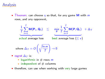
Analysis
Theorem: can choose so that, for any game M with m
rows, and any opponent, 1 T
T
M(Pt , Qt )
t=1
1 min P T
T
M(P, Qt ) + T
t=1
actual average loss where T = O
regret T is:
best average loss ( v ) 0
ln m T
logarithmic in # rows m independent of # columns
therefore, can use when working with very large games
62
![Slide: Solving a Game
suppose game M played repeatedly
[with Freund]
Mindy plays using MW on round t, Max chooses best response: Qt = arg max M(Pt , Q)
Q
let
1 P= T
T
Pt ,
t=1
1 Q= T
T
Qt
t=1
can prove that P and Q are T -approximate minmax and
maxmin strategies: max M(P, Q) v + T
Q
and min M(P, Q) v T
P](https://yosinski.com/mlss12/media/slides/MLSS-2012-Schapire-Theory-and-Applications-of-Boosting_063.png)
Solving a Game
suppose game M played repeatedly
[with Freund]
Mindy plays using MW on round t, Max chooses best response: Qt = arg max M(Pt , Q)
Q
let
1 P= T
T
Pt ,
t=1
1 Q= T
T
Qt
t=1
can prove that P and Q are T -approximate minmax and
maxmin strategies: max M(P, Q) v + T
Q
and min M(P, Q) v T
P
63
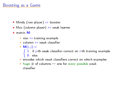
Boosting as a Game
Mindy (row player) booster Max (column player) weak learner matrix M:
row training example column weak classier M(i, j) = 1 if j-th weak classier correct on i-th training example 0 else encodes which weak classiers correct on which examples huge # of columns one for every possible weak classier
64
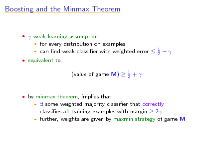
Boosting and the Minmax Theorem
-weak learning assumption:
for every distribution on examples can nd weak classier with weighted error
1 2
equivalent to:
(value of game M)
1 2
+
by minmax theorem, implies that:
some weighted majority classier that correctly classies all training examples with margin 2 further, weights are given by maxmin strategy of game M
65
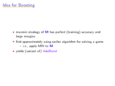
Idea for Boosting
maxmin strategy of M has perfect (training) accuracy and
large margins
nd approximately using earlier algorithm for solving a game
i.e., apply MW to M
yields (variant of) AdaBoost
66
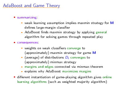
AdaBoost and Game Theory
summarizing:
weak learning assumption implies maxmin strategy for M denes large-margin classier AdaBoost nds maxmin strategy by applying general algorithm for solving games through repeated play
consequences:
weights on weak classiers converge to (approximately) maxmin strategy for game M (average) of distributions Dt converges to (approximately) minmax strategy margins and edges connected via minmax theorem explains why AdaBoost maximizes margins
dierent instantiation of game-playing algorithm gives online
learning algorithms (such as weighted majority algorithm)
67
Fundamental Perspectives
game theory loss minimization an information-geometric view
68
AdaBoost and Loss Minimization
many (most?) learning and statistical methods can be viewed
as minimizing loss (a.k.a. cost or objective) function measuring t to data: 2 e.g. least squares regression i (F (xi ) yi )
AdaBoost also minimizes a loss function helpful to understand because:
claries goal of algorithm and useful in proving convergence properties decoupling of algorithm from its objective means: faster algorithms possible for same objective same algorithm may generalize for new learning challenges
69
![Slide: What AdaBoost Minimizes
recall proof of training error bound:
training error(Hnal )
t
Zt
Zt = t e t + (1 t )e t = 2 t (1 t ) t chosen to minimize Zt ht chosen to minimize t same as minimizing Zt (since increasing in t on [0, 1/2]) equivalent to greedily minimizing
t
closer look:
so: both AdaBoost and weak learner minimize Zt on round t
Zt](https://yosinski.com/mlss12/media/slides/MLSS-2012-Schapire-Theory-and-Applications-of-Boosting_070.png)
What AdaBoost Minimizes
recall proof of training error bound:
training error(Hnal )
t
Zt
Zt = t e t + (1 t )e t = 2 t (1 t ) t chosen to minimize Zt ht chosen to minimize t same as minimizing Zt (since increasing in t on [0, 1/2]) equivalent to greedily minimizing
t
closer look:
so: both AdaBoost and weak learner minimize Zt on round t
Zt
70
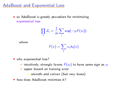
AdaBoost and Exponential Loss
so AdaBoost is greedy procedure for minimizing
exponential loss Zt =
t
1 m
exp(yi F (xi ))
i
where F (x) =
t
t ht (x)
why exponential loss?
intuitively, strongly favors F (xi ) to have same sign as yi upper bound on training error smooth and convex (but very loose)
how does AdaBoost minimize it?
71
![Slide: Coordinate Descent
{g1 , . . . , gN } = space of all weak classiers
N
[Breiman]
then can write F (x) =
t
t ht (x) =
j=1
j gj (x)
want to nd 1 , . . . , N to minimize
L(1 , . . . , N ) =
i
AdaBoost is actually doing coordinate descent on this
exp yi
j
j gj (xi )
optimization problem: initially, all j = 0 each round: choose one coordinate j (corresponding to ht ) and update (increment by t ) choose update causing biggest decrease in loss powerful technique for minimizing over huge space of functions](https://yosinski.com/mlss12/media/slides/MLSS-2012-Schapire-Theory-and-Applications-of-Boosting_072.png)
Coordinate Descent
{g1 , . . . , gN } = space of all weak classiers
N
[Breiman]
then can write F (x) =
t
t ht (x) =
j=1
j gj (x)
want to nd 1 , . . . , N to minimize
L(1 , . . . , N ) =
i
AdaBoost is actually doing coordinate descent on this
exp yi
j
j gj (xi )
optimization problem: initially, all j = 0 each round: choose one coordinate j (corresponding to ht ) and update (increment by t ) choose update causing biggest decrease in loss powerful technique for minimizing over huge space of functions
72
![Slide: Functional Gradient Descent
want to minimize
[Mason et al.][Friedman]
L(F ) = L(F (x1 ), . . . , F (xm )) =
i
exp(yi F (xi ))
say have current estimate F and want to improve to do gradient descent, would like update
F F F L(F )
but update restricted in class of weak classiers
F F + ht
so choose ht closest to F L(F ) equivalent to AdaBoost](https://yosinski.com/mlss12/media/slides/MLSS-2012-Schapire-Theory-and-Applications-of-Boosting_073.png)
Functional Gradient Descent
want to minimize
[Mason et al.][Friedman]
L(F ) = L(F (x1 ), . . . , F (xm )) =
i
exp(yi F (xi ))
say have current estimate F and want to improve to do gradient descent, would like update
F F F L(F )
but update restricted in class of weak classiers
F F + ht
so choose ht closest to F L(F ) equivalent to AdaBoost
73
![Slide: Estimating Conditional Probabilities
[Friedman, Hastie & Tibshirani]
often want to estimate probability that y = +1 given x AdaBoost minimizes (empirical version of):
Ex,y e yF (x) = Ex Pr [y = +1|x] e F (x) + Pr [y = 1|x] e F (x) where x, y random from true distribution
over all F , minimized when
F (x) = or
1 ln 2
Pr [y = +1|x] Pr [y = 1|x] 1 1 + e 2F (x)
Pr [y = +1|x] =
so, to convert F output by AdaBoost to probability estimate,
use same formula](https://yosinski.com/mlss12/media/slides/MLSS-2012-Schapire-Theory-and-Applications-of-Boosting_074.png)
Estimating Conditional Probabilities
[Friedman, Hastie & Tibshirani]
often want to estimate probability that y = +1 given x AdaBoost minimizes (empirical version of):
Ex,y e yF (x) = Ex Pr [y = +1|x] e F (x) + Pr [y = 1|x] e F (x) where x, y random from true distribution
over all F , minimized when
F (x) = or
1 ln 2
Pr [y = +1|x] Pr [y = 1|x] 1 1 + e 2F (x)
Pr [y = +1|x] =
so, to convert F output by AdaBoost to probability estimate,
use same formula
74
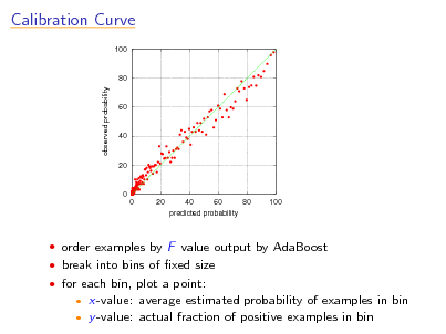
Calibration Curve
100
80
observed probability
60
40
20
0 0 20 40 60 80 100 predicted probability
order examples by F value output by AdaBoost break into bins of xed size for each bin, plot a point:
x-value: average estimated probability of examples in bin y -value: actual fraction of positive examples in bin
75
![Slide: A Synthetic Example
x [2, +2] uniform Pr [y = +1|x] = 2x
2
m = 500 training examples
1 1
0.5
0.5
0 -2 -1 0 1 2
0 -2 -1 0 1 2
if run AdaBoost with stumps and convert to probabilities,
result is poor extreme overtting](https://yosinski.com/mlss12/media/slides/MLSS-2012-Schapire-Theory-and-Applications-of-Boosting_076.png)
A Synthetic Example
x [2, +2] uniform Pr [y = +1|x] = 2x
2
m = 500 training examples
1 1
0.5
0.5
0 -2 -1 0 1 2
0 -2 -1 0 1 2
if run AdaBoost with stumps and convert to probabilities,
result is poor extreme overtting
76
![Slide: Regularization
AdaBoost minimizes
L() =
i
to avoid overtting, want to constrain to make solution
exp yi
j
j gj (xi )
smoother
(1 ) regularization:
minimize: L() subject to:
or:
1
B
minimize: L() +
other norms possible
1
1 (lasso) currently popular since encourages sparsity
[Tibshirani]](https://yosinski.com/mlss12/media/slides/MLSS-2012-Schapire-Theory-and-Applications-of-Boosting_077.png)
Regularization
AdaBoost minimizes
L() =
i
to avoid overtting, want to constrain to make solution
exp yi
j
j gj (xi )
smoother
(1 ) regularization:
minimize: L() subject to:
or:
1
B
minimize: L() +
other norms possible
1
1 (lasso) currently popular since encourages sparsity
[Tibshirani]
77
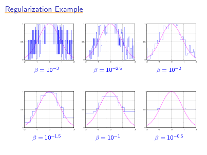
Regularization Example
1 1 1
0.5
0.5
0.5
0 -2 -1 0 1 2
0 -2 -1 0 1 2
0 -2 -1 0 1 2
=
103
=
102.5
=
102
1
1
1
0.5
0.5
0.5
0 -2 -1 0 1 2
0 -2 -1 0 1 2
0 -2 -1 0 1 2
=
101.5
=
101
=
100.5
78
![Slide: Regularization and AdaBoost
0.6 individual classifier weights 0.4 0.2 0 -0.2 -0.4 -0.6 0 0.5 1 1.5 2 2.5
[Hastie, Tibshirani & Friedman; Rosset, Zhu & Hastie]
0.6 individual classifier weights 0.4 0.2 0 -0.2 -0.4 -0.6 0 0.5 1 1.5 2 2.5
B Experiment 1: regularized
T Experiment 2: AdaBoost run
solution vectors plotted as function of B
with t xed to (small) solution vectors plotted as function of T
plots are identical! can prove under certain (but not all) conditions that results will be the same (as 0) [Zhao & Yu]](https://yosinski.com/mlss12/media/slides/MLSS-2012-Schapire-Theory-and-Applications-of-Boosting_079.png)
Regularization and AdaBoost
0.6 individual classifier weights 0.4 0.2 0 -0.2 -0.4 -0.6 0 0.5 1 1.5 2 2.5
[Hastie, Tibshirani & Friedman; Rosset, Zhu & Hastie]
0.6 individual classifier weights 0.4 0.2 0 -0.2 -0.4 -0.6 0 0.5 1 1.5 2 2.5
B Experiment 1: regularized
T Experiment 2: AdaBoost run
solution vectors plotted as function of B
with t xed to (small) solution vectors plotted as function of T
plots are identical! can prove under certain (but not all) conditions that results will be the same (as 0) [Zhao & Yu]
79
![Slide: Regularization and AdaBoost
suggests stopping AdaBoost early is akin to applying
1 -regularization
caveats:
does not strictly apply to AdaBoost (only variant) not helpful when boosting run to convergence (would correspond to very weak regularization)
in fact, in limit of vanishingly weak regularization (B ),
solution converges to maximum margin solution
[Rosset, Zhu & Hastie]](https://yosinski.com/mlss12/media/slides/MLSS-2012-Schapire-Theory-and-Applications-of-Boosting_080.png)
Regularization and AdaBoost
suggests stopping AdaBoost early is akin to applying
1 -regularization
caveats:
does not strictly apply to AdaBoost (only variant) not helpful when boosting run to convergence (would correspond to very weak regularization)
in fact, in limit of vanishingly weak regularization (B ),
solution converges to maximum margin solution
[Rosset, Zhu & Hastie]
80
![Slide: Benets of Loss-Minimization View
immediate generalization to other loss functions and learning
problems
e.g. squared error for regression e.g. logistic regression (by only changing one line of AdaBoost)
sensible approach for converting output of boosting into
conditional probability estimates
helpful connection to regularization basis for proving AdaBoost is statistically consistent
i.e., under right assumptions, converges to best possible classier [Bartlett & Traskin]](https://yosinski.com/mlss12/media/slides/MLSS-2012-Schapire-Theory-and-Applications-of-Boosting_081.png)
Benets of Loss-Minimization View
immediate generalization to other loss functions and learning
problems
e.g. squared error for regression e.g. logistic regression (by only changing one line of AdaBoost)
sensible approach for converting output of boosting into
conditional probability estimates
helpful connection to regularization basis for proving AdaBoost is statistically consistent
i.e., under right assumptions, converges to best possible classier [Bartlett & Traskin]
81
A Note of Caution
tempting (but incorrect!) to conclude:
AdaBoost is just an algorithm for minimizing exponential loss AdaBoost works only because of its loss function more powerful optimization techniques for same loss should work even better
incorrect because:
other algorithms that minimize exponential loss can give very poor generalization performance compared to AdaBoost
for example...
82
![Slide: An Experiment
data:
instances x uniform from {1, +1}10,000 label y = majority vote of three coordinates weak classier = single coordinate (or its negation) training set size m = 1000 algorithms (all provably minimize exponential loss): standard AdaBoost gradient descent on exponential loss AdaBoost, but in which weak classiers chosen at random results:
exp. loss 1010 1020 1040 10100
stand. AdaB. 0.0 [94] 0.0 [190] 0.0 [382] 0.0 [956]
% test error [# rounds] grad. desc. random AdaB. 40.7 [5] 44.0 [24,464] 40.8 [9] 41.6 [47,534] 40.8 [21] 40.9 [94,479] 40.8 [70] 40.3 [234,654]](https://yosinski.com/mlss12/media/slides/MLSS-2012-Schapire-Theory-and-Applications-of-Boosting_083.png)
An Experiment
data:
instances x uniform from {1, +1}10,000 label y = majority vote of three coordinates weak classier = single coordinate (or its negation) training set size m = 1000 algorithms (all provably minimize exponential loss): standard AdaBoost gradient descent on exponential loss AdaBoost, but in which weak classiers chosen at random results:
exp. loss 1010 1020 1040 10100
stand. AdaB. 0.0 [94] 0.0 [190] 0.0 [382] 0.0 [956]
% test error [# rounds] grad. desc. random AdaB. 40.7 [5] 44.0 [24,464] 40.8 [9] 41.6 [47,534] 40.8 [21] 40.9 [94,479] 40.8 [70] 40.3 [234,654]
83
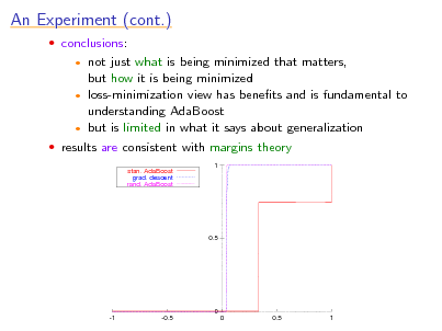
An Experiment (cont.)
conclusions:
not just what is being minimized that matters, but how it is being minimized loss-minimization view has benets and is fundamental to understanding AdaBoost but is limited in what it says about generalization results are consistent with margins theory
stan. AdaBoost grad. descent rand. AdaBoost 1
0.5
0 -1 -0.5 0 0.5 1
84
Fundamental Perspectives
game theory loss minimization an information-geometric view
85
A Dual Information-Geometric Perspective
loss minimization focuses on function computed by AdaBoost
(i.e., weights on weak classiers)
dual view: instead focus on distributions Dt
(i.e., weights on examples)
dual perspective combines geometry and information theory exposes underlying mathematical structure basis for proving convergence
86
![Slide: An Iterative-Projection Algorithm
say want to nd point closest to x0 in set
P = { intersection of N hyperplanes }
algorithm:
[Bregman; Censor & Zenios]
start at x0 repeat: pick a hyperplane and project onto it
P x0
if P = , under general conditions, will converge correctly](https://yosinski.com/mlss12/media/slides/MLSS-2012-Schapire-Theory-and-Applications-of-Boosting_087.png)
An Iterative-Projection Algorithm
say want to nd point closest to x0 in set
P = { intersection of N hyperplanes }
algorithm:
[Bregman; Censor & Zenios]
start at x0 repeat: pick a hyperplane and project onto it
P x0
if P = , under general conditions, will converge correctly
87
![Slide: AdaBoost is an Iterative-Projection Algorithm
points = distributions Dt over training examples distance = relative entropy:
[Kivinen & Warmuth]
RE (P
Q) =
i
P(i) ln
P(i) Q(i)
reference point x0 = uniform distribution hyperplanes dened by all possible weak classiers gj :
D(i)yi gj (xi ) = 0 Pr [gj (xi ) = yi ] =
i iD
1 2
intuition: looking for hardest distribution](https://yosinski.com/mlss12/media/slides/MLSS-2012-Schapire-Theory-and-Applications-of-Boosting_088.png)
AdaBoost is an Iterative-Projection Algorithm
points = distributions Dt over training examples distance = relative entropy:
[Kivinen & Warmuth]
RE (P
Q) =
i
P(i) ln
P(i) Q(i)
reference point x0 = uniform distribution hyperplanes dened by all possible weak classiers gj :
D(i)yi gj (xi ) = 0 Pr [gj (xi ) = yi ] =
i iD
1 2
intuition: looking for hardest distribution
88
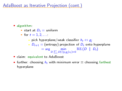
AdaBoost as Iterative Projection (cont.)
algorithm:
start at D1 = uniform for t = 1, 2, . . .: pick hyperplane/weak classier ht gj Dt+1 = (entropy) projection of Dt onto hyperplane = arg min RE (D Dt )
D:
i
D(i)yi gj (xi )=0
claim: equivalent to AdaBoost further: choosing ht with minimum error choosing farthest
hyperplane
89
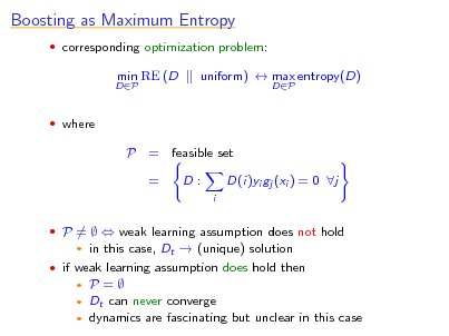
Boosting as Maximum Entropy
corresponding optimization problem:
DP
min RE (D
uniform) max entropy(D)
DP
where
P = feasible set = D:
i
D(i)yi gj (xi ) = 0 j
P = weak learning assumption does not hold
in this case, Dt (unique) solution
if weak learning assumption does hold then
P= Dt can never converge dynamics are fascinating but unclear in this case
90
![Slide: Visualizing Dynamics
plot one circle for each round t:
[with Rudin & Daubechies]
center at (Dt (1), Dt (2)) radius t (color also varies with t)
t=3
0.5
11111 00000 11111 00000 11111 00000 11111 00000 11111 00000 11111 00000 11111 00000 11111 00000 11111 00000 11111 00000 11111 00000 11111 00000 11111 00000 11111 00000 11111 00000
0.4
t=6
11111 00000 11111 00000 11111 00000 11111 00000 11111 00000 11111 00000 11111 00000 11111 00000
d
D (2) t
t,2
t=1 t=4 t=5
0.2
111111 000000 0.3 d 111111 000000 0.4 111111 000000 t,1 111111 000000 111111 000000 111111 000000 111111 000000
t=2
0.2
D (1) t
0.5
in all cases examined, appears to converge eventually to cycle
open if always true](https://yosinski.com/mlss12/media/slides/MLSS-2012-Schapire-Theory-and-Applications-of-Boosting_091.png)
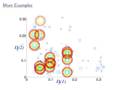
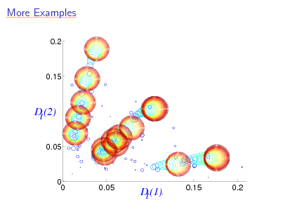
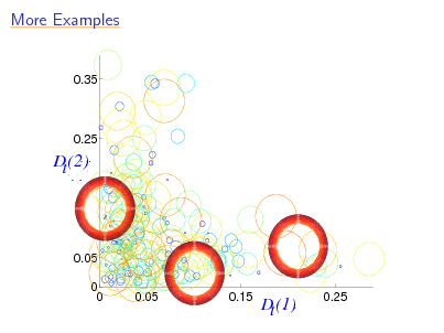
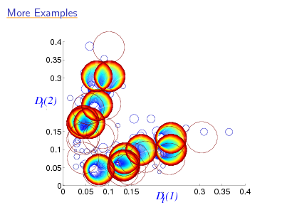
Visualizing Dynamics
plot one circle for each round t:
[with Rudin & Daubechies]
center at (Dt (1), Dt (2)) radius t (color also varies with t)
t=3
0.5
11111 00000 11111 00000 11111 00000 11111 00000 11111 00000 11111 00000 11111 00000 11111 00000 11111 00000 11111 00000 11111 00000 11111 00000 11111 00000 11111 00000 11111 00000
0.4
t=6
11111 00000 11111 00000 11111 00000 11111 00000 11111 00000 11111 00000 11111 00000 11111 00000
d
D (2) t
t,2
t=1 t=4 t=5
0.2
111111 000000 0.3 d 111111 000000 0.4 111111 000000 t,1 111111 000000 111111 000000 111111 000000 111111 000000
t=2
0.2
D (1) t
0.5
in all cases examined, appears to converge eventually to cycle
open if always true
91
More Examples
0.35
0.25
111111 000000 111111 000000 111111 000000 111111 000000 111111 000000 111111 000000 111111 000000 111111 000000 111111 000000 111111 000000
D (2) t
dt,2
0.1
0 0
111111 0.1 000000 111111 000000 d 111111 000000 111111 000000 111111 000000
111111 000000 111111 000000
D (1) t t,1
0.2
0.3
92
More Examples
0.2
0.15
111111 000000 111111 000000 111111 000000 111111 000000 111111 000000 111111 000000 111111 000000 111111 000000 111111 000000 111111 000000
d
D (2) t
0.05
t,12
0 0
0.05
d (1) D t,11 t
11111 00000 11111 00000 11111 00000 11111 00000 11111 00000 11111 00000 11111 00000
0.15
0.2
93
More Examples
0.35
111111 000000 111111 000000 111111 000000 111111 000000 111111 000000 111111 000000 111111 000000 111111 000000 111111 000000
0.25
d
D (2) t
0.05 0 0 0.05 0.15
11111 00000 11111 00000 11111 00000 11111 00000 11111 00000 11111 00000
t,2
Ddt,1 t (1)
0.25
94
More Examples
0.4 0.35 0.3
11111 00000 11111 00000 11111 00000 11111 00000 11111 00000 11111 00000 11111 00000 11111 00000 11111 00000 11111 00000
d
D (2) t
0.15 0.1 0.05 0 0 0.05 0.1 0.15
11111 00000 11111 00000 11111 00000 11111 00000 t,1 11111 00000 11111 00000
t,2
d D (1) t
0.3
0.35
0.4
95
![Slide: Unifying the Two Cases
two distinct cases:
[with Collins & Singer]
weak learning assumption holds P = dynamics unclear weak learning assumption does not hold P = can prove convergence of Dt s to unify: work instead with unnormalized versions of Dt s Dt (i) exp(t yi ht (xi )) standard AdaBoost: Dt+1 (i) = normalization instead: dt+1 (i) = dt (i) exp(t yi ht (xi )) dt+1 (i) Dt+1 (i) = normalization
algorithm is unchanged](https://yosinski.com/mlss12/media/slides/MLSS-2012-Schapire-Theory-and-Applications-of-Boosting_096.png)
Unifying the Two Cases
two distinct cases:
[with Collins & Singer]
weak learning assumption holds P = dynamics unclear weak learning assumption does not hold P = can prove convergence of Dt s to unify: work instead with unnormalized versions of Dt s Dt (i) exp(t yi ht (xi )) standard AdaBoost: Dt+1 (i) = normalization instead: dt+1 (i) = dt (i) exp(t yi ht (xi )) dt+1 (i) Dt+1 (i) = normalization
algorithm is unchanged
96
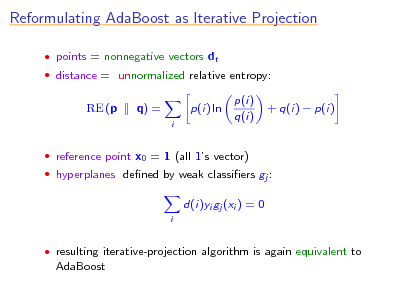
Reformulating AdaBoost as Iterative Projection
points = nonnegative vectors dt distance = unnormalized relative entropy:
RE (p
q) =
i
p(i) ln
p(i) q(i)
+ q(i) p(i)
reference point x0 = 1 (all 1s vector) hyperplanes dened by weak classiers gj :
d(i)yi gj (xi ) = 0
i
resulting iterative-projection algorithm is again equivalent to
AdaBoost
97
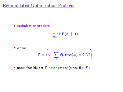
Reformulated Optimization Problem
optimization problem:
min RE (d
dP
1)
where
P=
d:
i
d(i)yi gj (xi ) = 0 j
note: feasible set P never empty (since 0 P)
98
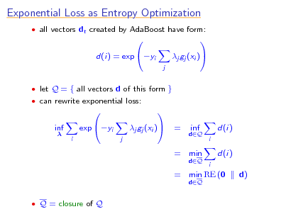
Exponential Loss as Entropy Optimization
all vectors dt created by AdaBoost have form:
d(i) = exp yi
j
j gj (xi )
let Q = { all vectors d of this form } can rewrite exponential loss:
inf
i
exp yi
j
j gj (xi )
=
dQ
inf
d(i)
i
= min
dQ dQ i
d(i) d)
= min RE (0
Q = closure of Q
99
![Slide: Duality
[Della Pietra, Della Pietra & Laerty]
presented two optimization problems:
min RE (d
dP
1) d)
min RE (0
dQ
which is AdaBoost solving? Both! problems have same solution moreover: solution given by unique point in P Q problems are convex duals of each other](https://yosinski.com/mlss12/media/slides/MLSS-2012-Schapire-Theory-and-Applications-of-Boosting_100.png)
Duality
[Della Pietra, Della Pietra & Laerty]
presented two optimization problems:
min RE (d
dP
1) d)
min RE (0
dQ
which is AdaBoost solving? Both! problems have same solution moreover: solution given by unique point in P Q problems are convex duals of each other
100
![Slide: Convergence of AdaBoost
can use to prove AdaBoost converges to common solution of
both problems: can argue that d = lim dt is in P vectors dt are in Q always d Q d P Q d solves both optimization problems
so:
AdaBoost minimizes exponential loss exactly characterizes limit of unnormalized distributions likewise for normalized distributions when weak learning assumption does not hold
also, provides additional link to logistic regression
only need slight change in optimization problem
[with Collins & Singer; Lebannon & Laerty]](https://yosinski.com/mlss12/media/slides/MLSS-2012-Schapire-Theory-and-Applications-of-Boosting_101.png)
Convergence of AdaBoost
can use to prove AdaBoost converges to common solution of
both problems: can argue that d = lim dt is in P vectors dt are in Q always d Q d P Q d solves both optimization problems
so:
AdaBoost minimizes exponential loss exactly characterizes limit of unnormalized distributions likewise for normalized distributions when weak learning assumption does not hold
also, provides additional link to logistic regression
only need slight change in optimization problem
[with Collins & Singer; Lebannon & Laerty]
101
Practical Extensions
multiclass classication ranking problems condence-rated predictions
102
Practical Extensions
multiclass classication ranking problems condence-rated predictions
103
![Slide: Multiclass Problems
say y Y where |Y | = k direct approach (AdaBoost.M1):
[with Freund]
ht : X Y Dt+1 (i) = Dt (i) Zt e t e t
y Y
if yi = ht (xi ) if yi = ht (xi ) t
t:ht (x)=y
Hnal (x) = arg max
can prove same bound on error if t : t 1/2
in practice, not usually a problem for strong weak learners (e.g., C4.5) signicant problem for weak weak learners (e.g., decision stumps) instead, reduce to binary](https://yosinski.com/mlss12/media/slides/MLSS-2012-Schapire-Theory-and-Applications-of-Boosting_104.png)
Multiclass Problems
say y Y where |Y | = k direct approach (AdaBoost.M1):
[with Freund]
ht : X Y Dt+1 (i) = Dt (i) Zt e t e t
y Y
if yi = ht (xi ) if yi = ht (xi ) t
t:ht (x)=y
Hnal (x) = arg max
can prove same bound on error if t : t 1/2
in practice, not usually a problem for strong weak learners (e.g., C4.5) signicant problem for weak weak learners (e.g., decision stumps) instead, reduce to binary
104
![Slide: The One-Against-All Approach
break k-class problem into k binary problems and
solve each separately
say possible labels are Y = { , , , }
x1 x2 x3 x4 x5
x1 x2 x3 x4 x5
+
x1 x2 x3 x4 x5
+ +
x1 x2 x3 x4 x5
+
x1 x2 x3 x4 x5
+
to classify new example, choose label predicted to be most
positive
AdaBoost.MH problem: not robust to errors in predictions [with Singer]](https://yosinski.com/mlss12/media/slides/MLSS-2012-Schapire-Theory-and-Applications-of-Boosting_105.png)
The One-Against-All Approach
break k-class problem into k binary problems and
solve each separately
say possible labels are Y = { , , , }
x1 x2 x3 x4 x5
x1 x2 x3 x4 x5
+
x1 x2 x3 x4 x5
+ +
x1 x2 x3 x4 x5
+
x1 x2 x3 x4 x5
+
to classify new example, choose label predicted to be most
positive
AdaBoost.MH problem: not robust to errors in predictions [with Singer]
105
![Slide: Using Output Codes
[with Allwein & Singer][Dietterich & Bakiri]
M
reduce to binary using
coding matrix M
rows of M code words
1 + + + 4 + + +
2 + + x1 x2 x3 x4 x5
3 + + + 5 + + +
4 + +
5 + +
1 x1 x2 x3 x4 x5 x1 x2 x3 x4 x5 + + + x1 x2 x3 x4 x5
2 + + x1 x2 x3 x4 x5
3 + + + + x1 x2 x3 x4 x5
to classify new example, choose closest row of M](https://yosinski.com/mlss12/media/slides/MLSS-2012-Schapire-Theory-and-Applications-of-Boosting_106.png)
Using Output Codes
[with Allwein & Singer][Dietterich & Bakiri]
M
reduce to binary using
coding matrix M
rows of M code words
1 + + + 4 + + +
2 + + x1 x2 x3 x4 x5
3 + + + 5 + + +
4 + +
5 + +
1 x1 x2 x3 x4 x5 x1 x2 x3 x4 x5 + + + x1 x2 x3 x4 x5
2 + + x1 x2 x3 x4 x5
3 + + + + x1 x2 x3 x4 x5
to classify new example, choose closest row of M
106
Output Codes (continued)
if rows of M far from one another,
will be highly robust to errors
potentially much faster when k (# of classes) large disadvantage:
binary problems may be unnatural and hard to solve
107
Practical Extensions
multiclass classication ranking problems condence-rated predictions
108
![Slide: Ranking Problems
[with Freund, Iyer & Singer]
goal: learn to rank objects (e.g., movies, webpages, etc.) from
examples
can reduce to multiple binary questions of form:
is or is not object A preferred to object B?
now apply (binary) AdaBoost RankBoost](https://yosinski.com/mlss12/media/slides/MLSS-2012-Schapire-Theory-and-Applications-of-Boosting_109.png)
Ranking Problems
[with Freund, Iyer & Singer]
goal: learn to rank objects (e.g., movies, webpages, etc.) from
examples
can reduce to multiple binary questions of form:
is or is not object A preferred to object B?
now apply (binary) AdaBoost RankBoost
109
![Slide: Application: Finding Cancer Genes
[Agarwal & Sengupta]
examples are genes (described by microarray vectors) want to rank genes from most to least relevant to leukemia data sizes:
7129 genes total 10 known relevant 157 known irrelevant](https://yosinski.com/mlss12/media/slides/MLSS-2012-Schapire-Theory-and-Applications-of-Boosting_110.png)
Application: Finding Cancer Genes
[Agarwal & Sengupta]
examples are genes (described by microarray vectors) want to rank genes from most to least relevant to leukemia data sizes:
7129 genes total 10 known relevant 157 known irrelevant
110
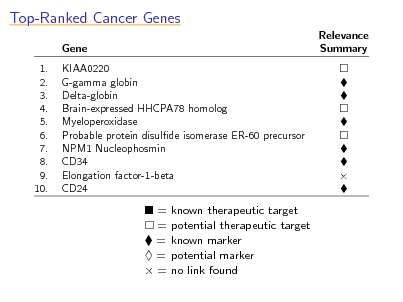
Top-Ranked Cancer Genes
Gene 1. 2. 3. 4. 5. 6. 7. 8. 9. 10. KIAA0220 G-gamma globin Delta-globin Brain-expressed HHCPA78 homolog Myeloperoxidase Probable protein disulde isomerase ER-60 precursor NPM1 Nucleophosmin CD34 Elongation factor-1-beta CD24 Relevance Summary
= = = = =
known therapeutic target potential therapeutic target known marker potential marker no link found
111
Practical Extensions
multiclass classication ranking problems condence-rated predictions
112
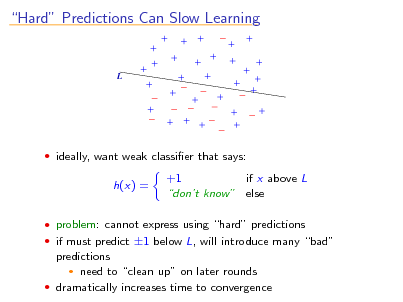
Hard Predictions Can Slow Learning
L
ideally, want weak classier that says:
h(x) =
+1 if x above L dont know else
problem: cannot express using hard predictions if must predict 1 below L, will introduce many bad
predictions need to clean up on later rounds dramatically increases time to convergence
113
![Slide: Condence-Rated Predictions
[with Singer]
useful to allow weak classiers to assign condences to
predictions
formally, allow ht : X R
sign(ht (x)) = prediction |ht (x)| = condence
use identical update:
Dt+1 (i) =
Dt (i) exp(t yi ht (xi )) Zt
and identical rule for combining weak classiers
question: how to choose t and ht on each round](https://yosinski.com/mlss12/media/slides/MLSS-2012-Schapire-Theory-and-Applications-of-Boosting_114.png)
Condence-Rated Predictions
[with Singer]
useful to allow weak classiers to assign condences to
predictions
formally, allow ht : X R
sign(ht (x)) = prediction |ht (x)| = condence
use identical update:
Dt+1 (i) =
Dt (i) exp(t yi ht (xi )) Zt
and identical rule for combining weak classiers
question: how to choose t and ht on each round
114
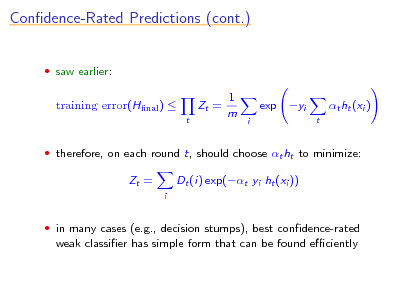
Condence-Rated Predictions (cont.)
saw earlier:
training error(Hnal )
t
Zt =
1 m
exp yi
i t
t ht (xi )
therefore, on each round t, should choose t ht to minimize:
Zt =
i
Dt (i) exp(t yi ht (xi ))
in many cases (e.g., decision stumps), best condence-rated
weak classier has simple form that can be found eciently
115
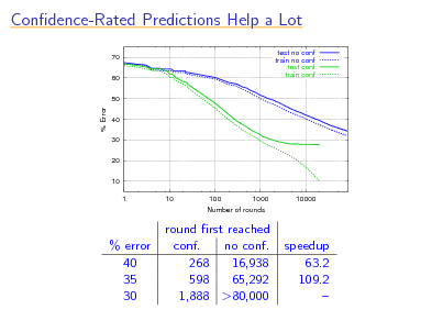
Condence-Rated Predictions Help a Lot
70 60 50 test no conf train no conf test conf train conf
% Error
40 30 20 10 1 10 100 1000 Number of rounds 10000
% error 40 35 30
round rst reached conf. no conf. 268 16,938 598 65,292 1,888 >80,000
speedup 63.2 109.2
116
![Slide: Application: Boosting for Text Categorization
[with Singer]
weak classiers: very simple weak classiers that test on
simple patterns, namely, (sparse) n-grams nd parameter t and rule ht of given form which minimize Zt use eciently implemented exhaustive search
How may I help you data:
7844 training examples 1000 test examples categories: AreaCode, AttService, BillingCredit, CallingCard, Collect, Competitor, DialForMe, Directory, HowToDial, PersonToPerson, Rate, ThirdNumber, Time, TimeCharge, Other.](https://yosinski.com/mlss12/media/slides/MLSS-2012-Schapire-Theory-and-Applications-of-Boosting_117.png)
Application: Boosting for Text Categorization
[with Singer]
weak classiers: very simple weak classiers that test on
simple patterns, namely, (sparse) n-grams nd parameter t and rule ht of given form which minimize Zt use eciently implemented exhaustive search
How may I help you data:
7844 training examples 1000 test examples categories: AreaCode, AttService, BillingCredit, CallingCard, Collect, Competitor, DialForMe, Directory, HowToDial, PersonToPerson, Rate, ThirdNumber, Time, TimeCharge, Other.
117
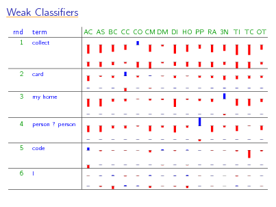
Weak Classiers
rnd
1
term
collect
AC AS BC CC CO CM DM DI HO PP RA 3N TI TC OT
2
card
3
my home
4
person ? person
5
code
6
I
118
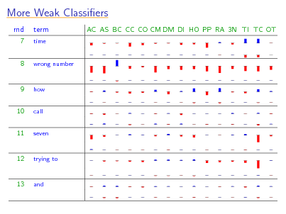
More Weak Classiers
rnd
7
term
time
AC AS BC CC CO CM DM DI HO PP RA 3N TI TC OT
8
wrong number
9 10 11
how call seven
12
trying to
13
and
119
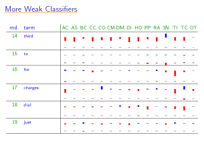
More Weak Classiers
rnd
14
term
third
AC AS BC CC CO CM DM DI HO PP RA 3N TI TC OT
15 16
to for
17
charges
18
dial
19
just
120
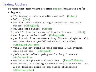
Finding Outliers
examples with most weight are often outliers (mislabeled and/or ambiguous)
Im trying to make a credit card call (Collect) hello (Rate) yes Id like to make a long distance collect call please (CallingCard) calling card please (Collect) yeah Id like to use my calling card number (Collect) can I get a collect call (CallingCard) yes I would like to make a long distant telephone call and have the charges billed to another number (CallingCard DialForMe) yeah I can not stand it this morning I did oversea (BillingCredit) call is so bad yeah special offers going on for long distance (AttService Rate) mister allen please william allen (PersonToPerson) yes maam I Im trying to make a long distance call to a non dialable point in san miguel philippines (AttService Other)
121
Advanced Topics
optimal accuracy optimal eciency boosting in continuous time
122
Advanced Topics
optimal accuracy optimal eciency boosting in continuous time
123
![Slide: Optimal Accuracy
noise or uncertainty
[Bartlett & Traskin]
usually, impossible to get perfect accuracy due to intrinsic Bayes optimal error = best possible error of any classier
usually > 0
can prove AdaBoosts classier converges to Bayes optimal if:
enough data run for many (but not too many) rounds weak classiers suciently rich
universally consistent related results: [Jiang], [Lugosi & Vayatis], [Zhang & Yu], . . . means:
AdaBoost can (theoretically) learn optimally even in noisy settings but: does not explain why works when run for very many rounds](https://yosinski.com/mlss12/media/slides/MLSS-2012-Schapire-Theory-and-Applications-of-Boosting_124.png)
Optimal Accuracy
noise or uncertainty
[Bartlett & Traskin]
usually, impossible to get perfect accuracy due to intrinsic Bayes optimal error = best possible error of any classier
usually > 0
can prove AdaBoosts classier converges to Bayes optimal if:
enough data run for many (but not too many) rounds weak classiers suciently rich
universally consistent related results: [Jiang], [Lugosi & Vayatis], [Zhang & Yu], . . . means:
AdaBoost can (theoretically) learn optimally even in noisy settings but: does not explain why works when run for very many rounds
124
![Slide: Boosting and Noise
[Long & Servedio]
can construct data source on which AdaBoost fails miserably
with even tiny amount of noise (say, 1%) Bayes optimal error = 1% (obtainable by classier of same form as AdaBoost) AdaBoost provably has error 50%
holds even if:
given unlimited training data use any method for minimizing exponential loss
also holds:
for most other convex losses even if add regularization e.g. applies to SVMs, logistic regression, . . .](https://yosinski.com/mlss12/media/slides/MLSS-2012-Schapire-Theory-and-Applications-of-Boosting_125.png)
Boosting and Noise
[Long & Servedio]
can construct data source on which AdaBoost fails miserably
with even tiny amount of noise (say, 1%) Bayes optimal error = 1% (obtainable by classier of same form as AdaBoost) AdaBoost provably has error 50%
holds even if:
given unlimited training data use any method for minimizing exponential loss
also holds:
for most other convex losses even if add regularization e.g. applies to SVMs, logistic regression, . . .
125
![Slide: Boosting and Noise (cont.)
shows:
consistency result can fail badly if weak classiers not rich enough AdaBoost (and lots of other loss-based methods) susceptible to noise regularization might not help
how to handle noise?
on real-world datasets, AdaBoost often works anyway various theoretical algorithms based on branching programs (e.g., [Kalai & Servedio], [Long & Servedio])](https://yosinski.com/mlss12/media/slides/MLSS-2012-Schapire-Theory-and-Applications-of-Boosting_126.png)
Boosting and Noise (cont.)
shows:
consistency result can fail badly if weak classiers not rich enough AdaBoost (and lots of other loss-based methods) susceptible to noise regularization might not help
how to handle noise?
on real-world datasets, AdaBoost often works anyway various theoretical algorithms based on branching programs (e.g., [Kalai & Servedio], [Long & Servedio])
126
Advanced Topics
optimal accuracy optimal eciency boosting in continuous time
127
![Slide: Optimal Eciency
for AdaBoost, saw: training error e 2
2T
[Freund]
is AdaBoost most ecient boosting algorithm?
no!
given T rounds and -weak learning assumption,
boost-by-majority (BBM) algorithm is provably exactly best possible:
T /2
training error
j=0
T j
1 2
+
j
1 2
T j
(probability of T /2 heads in T coin ips if probability of heads = 1 + ) 2
AdaBoosts training error is like Cherno approximation of
BBMs](https://yosinski.com/mlss12/media/slides/MLSS-2012-Schapire-Theory-and-Applications-of-Boosting_128.png)
Optimal Eciency
for AdaBoost, saw: training error e 2
2T
[Freund]
is AdaBoost most ecient boosting algorithm?
no!
given T rounds and -weak learning assumption,
boost-by-majority (BBM) algorithm is provably exactly best possible:
T /2
training error
j=0
T j
1 2
+
j
1 2
T j
(probability of T /2 heads in T coin ips if probability of heads = 1 + ) 2
AdaBoosts training error is like Cherno approximation of
BBMs
128
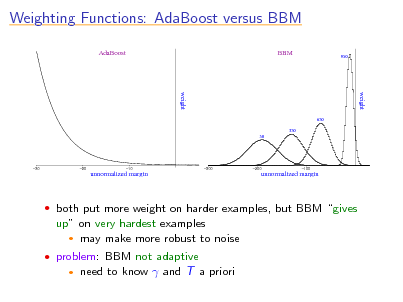
Weighting Functions: AdaBoost versus BBM
AdaBoost BBM
950
weight
650 350 50
weight
30
20
unnormalized margin
s
10
300
200
unnormalized margin
s
100
both put more weight on harder examples, but BBM gives
up on very hardest examples may make more robust to noise
problem: BBM not adaptive
need to know and T a priori
129
Advanced Topics
optimal accuracy optimal eciency boosting in continuous time
130
![Slide: Boosting in Continuous Time
[Freund]
idea: let get very small so that -weak learning assumption
eventually satised
need to make T correspondingly large if scale time to begin at = 0 and end at = 1, then each
boosting round takes time 1/T
in limit T , boosting is happening in continuous time](https://yosinski.com/mlss12/media/slides/MLSS-2012-Schapire-Theory-and-Applications-of-Boosting_131.png)
Boosting in Continuous Time
[Freund]
idea: let get very small so that -weak learning assumption
eventually satised
need to make T correspondingly large if scale time to begin at = 0 and end at = 1, then each
boosting round takes time 1/T
in limit T , boosting is happening in continuous time
131
![Slide: BrownBoost
algorithm has sensible limit called BrownBoost
(due to connection to Brownian motion)
harder to implement, but potentially more resistant to noise
and outliers, e.g.: dataset letter noise 0% 10% 20% 0% 10% 20% AdaBoost 3.7 10.8 15.7 4.9 12.1 21.3 BrownBoost 4.2 7.0 10.5 5.2 6.2 7.4
satimage
[Cheamanunkul, Ettinger & Freund]](https://yosinski.com/mlss12/media/slides/MLSS-2012-Schapire-Theory-and-Applications-of-Boosting_132.png)
BrownBoost
algorithm has sensible limit called BrownBoost
(due to connection to Brownian motion)
harder to implement, but potentially more resistant to noise
and outliers, e.g.: dataset letter noise 0% 10% 20% 0% 10% 20% AdaBoost 3.7 10.8 15.7 4.9 12.1 21.3 BrownBoost 4.2 7.0 10.5 5.2 6.2 7.4
satimage
[Cheamanunkul, Ettinger & Freund]
132
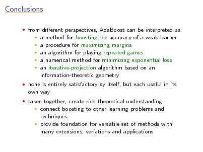
Conclusions
from dierent perspectives, AdaBoost can be interpreted as:
a method for boosting the accuracy of a weak learner a procedure for maximizing margins an algorithm for playing repeated games a numerical method for minimizing exponential loss an iterative-projection algorithm based on an information-theoretic geometry
none is entirely satisfactory by itself, but each useful in its
own way
taken together, create rich theoretical understanding
connect boosting to other learning problems and techniques provide foundation for versatile set of methods with many extensions, variations and applications
133
References
Robert E. Schapire and Yoav Freund.
Boosting: Foundations and Algorithms. MIT Press, 2012.
134