Convex Optimization: Modeling and Algorithms
Lieven Vandenberghe Electrical Engineering Department, UC Los Angeles

Tutorial lectures, 21st Machine Learning Summer School Kyoto, August 29-30, 2012

Convex optimization MLSS 2012

Introduction

mathematical optimization linear and convex optimization recent history

1

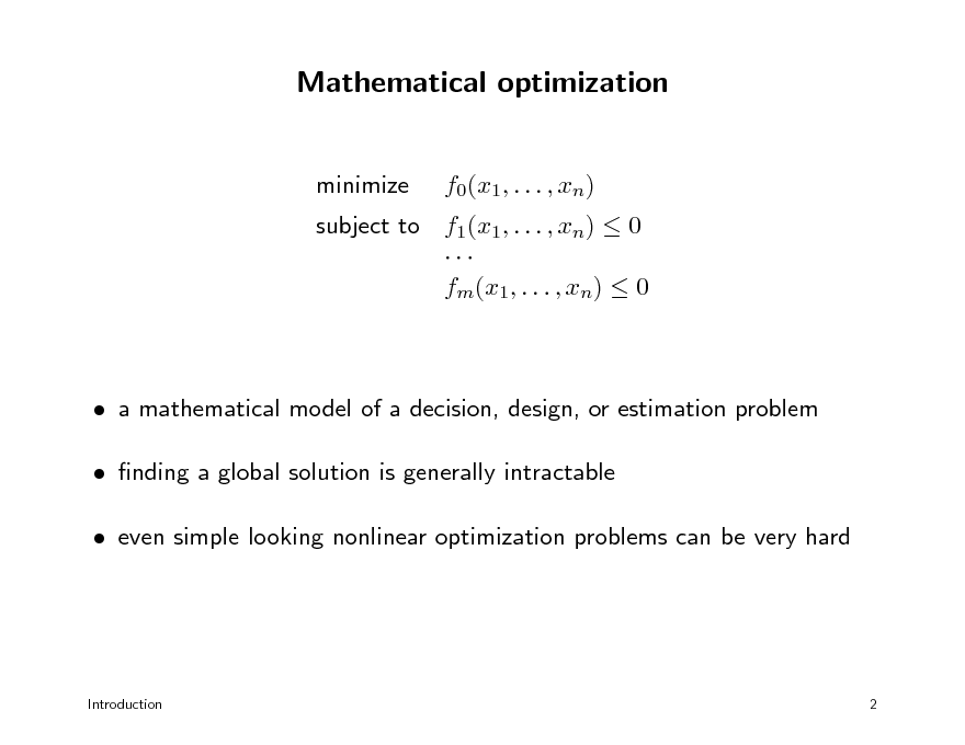
Mathematical optimization
minimize f0(x1, . . . , xn)

subject to f1(x1, . . . , xn) 0 fm(x1, . . . , xn) 0

a mathematical model of a decision, design, or estimation problem nding a global solution is generally intractable even simple looking nonlinear optimization problems can be very hard

Introduction

2

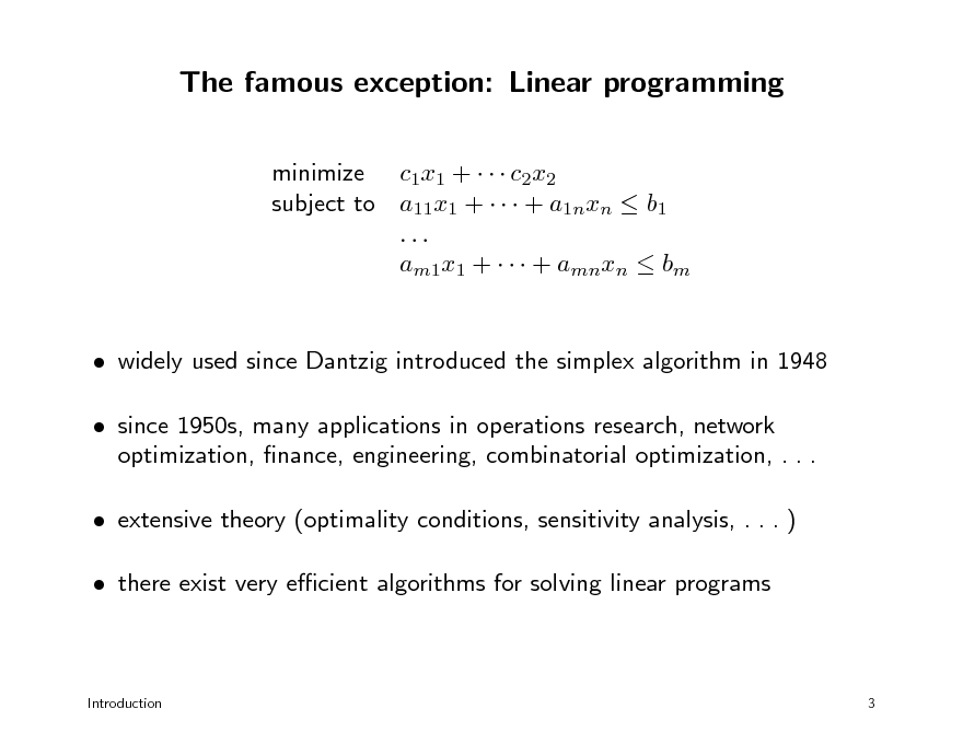
The famous exception: Linear programming
minimize c1x1 + c2x2 subject to a11x1 + + a1nxn b1 ... am1x1 + + amnxn bm widely used since Dantzig introduced the simplex algorithm in 1948 since 1950s, many applications in operations research, network optimization, nance, engineering, combinatorial optimization, . . . extensive theory (optimality conditions, sensitivity analysis, . . . ) there exist very ecient algorithms for solving linear programs

Introduction

3

Convex optimization problem
minimize f0(x) subject to fi(x) 0,

i = 1, . . . , m

objective and constraint functions are convex: for 0 1 fi(x + (1 )y) fi(x) + (1 )fi(y) can be solved globally, with similar (polynomial-time) complexity as LPs surprisingly many problems can be solved via convex optimization provides tractable heuristics and relaxations for non-convex problems

Introduction

4

History

1940s: linear programming minimize cT x subject to aT x bi, i 1950s: quadratic programming 1960s: geometric programming 1990s: semidenite programming, second-order cone programming, quadratically constrained quadratic programming, robust optimization, sum-of-squares programming, . . . i = 1, . . . , m

Introduction

5

New applications since 1990

linear matrix inequality techniques in control support vector machine training via quadratic programming semidenite programming relaxations in combinatorial optimization circuit design via geometric programming 1-norm optimization for sparse signal reconstruction applications in structural optimization, statistics, signal processing, communications, image processing, computer vision, quantum information theory, nance, power distribution, . . .

Introduction

6

Advances in convex optimization algorithms
interior-point methods 1984 (Karmarkar): rst practical polynomial-time algorithm for LP 1984-1990: ecient implementations for large-scale LPs around 1990 (Nesterov & Nemirovski): polynomial-time interior-point methods for nonlinear convex programming since 1990: extensions and high-quality software packages rst-order algorithms fast gradient methods, based on Nesterovs methods from 1980s extend to certain nondierentiable or constrained problems multiplier methods for large-scale and distributed optimization
Introduction 7

Overview

1. Basic theory and convex modeling convex sets and functions common problem classes and applications 2. Interior-point methods for conic optimization conic optimization barrier methods symmetric primal-dual methods 3. First-order methods (proximal) gradient algorithms dual techniques and multiplier methods

Convex optimization MLSS 2012

Convex sets and functions

convex sets convex functions operations that preserve convexity

Convex set
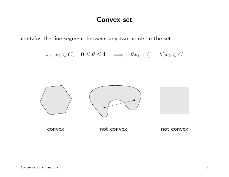
contains the line segment between any two points in the set x1, x2 C, 01 = x1 + (1 )x2 C

convex

not convex

not convex

Convex sets and functions

8

Basic examples
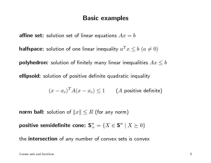
ane set: solution set of linear equations Ax = b halfspace: solution of one linear inequality aT x b (a = 0) polyhedron: solution of nitely many linear inequalities Ax b ellipsoid: solution of positive denite quadratic inquality (x xc)T A(x xc) 1 (A positive denite)

norm ball: solution of x R (for any norm) positive semidenite cone: Sn = {X Sn | X + 0}

the intersection of any number of convex sets is convex
Convex sets and functions 9

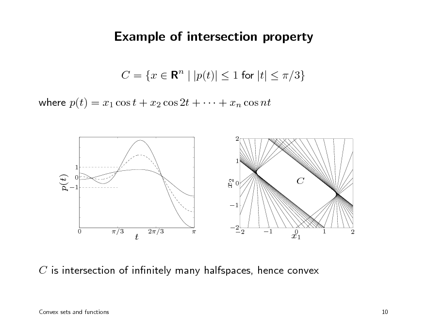
Example of intersection property
C = {x Rn | |p(t)| 1 for |t| /3} where p(t) = x1 cos t + x2 cos 2t + + xn cos nt
2 1

1

p(t)

x2

0 1

0

C

1 2 2

0

/3

t

2/3

1

0 x1

1

2

C is intersection of innitely many halfspaces, hence convex

Convex sets and functions

10

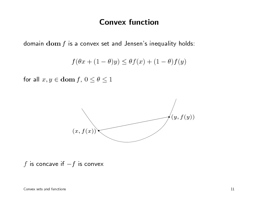
Convex function
domain dom f is a convex set and Jensens inequality holds: f (x + (1 )y) f (x) + (1 )f (y) for all x, y dom f , 0 1

(y, f (y)) (x, f (x))

f is concave if f is convex
Convex sets and functions 11

Examples
linear and ane functions are convex and concave exp x, log x, x log x are convex x is convex for x > 0 and 1 or 0; |x| is convex for 1 norms are convex quadratic-over-linear function xT x/t is convex in x, t for t > 0 geometric mean (x1x2 xn)1/n is concave for x 0 log det X is concave on set of positive denite matrices log(ex1 + exn ) is convex
Convex sets and functions 12

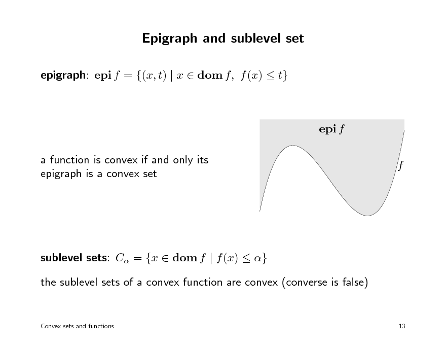
Epigraph and sublevel set
epigraph: epi f = {(x, t) | x dom f, f (x) t}

epi f a function is convex if and only its epigraph is a convex set f

sublevel sets: C = {x dom f | f (x) } the sublevel sets of a convex function are convex (converse is false)

Convex sets and functions

13

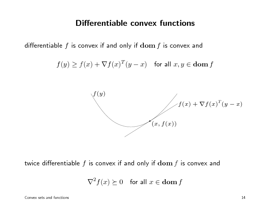
Dierentiable convex functions
dierentiable f is convex if and only if dom f is convex and f (y) f (x) + f (x)T (y x)
f (y) f (x) + f (x)T (y x) (x, f (x))

for all x, y dom f

twice dierentiable f is convex if and only if dom f is convex and 2f (x)
Convex sets and functions

0 for all x dom f
14

Establishing convexity of a function

1. verify denition 2. for twice dierentiable functions, show 2f (x) 0

3. show that f is obtained from simple convex functions by operations that preserve convexity nonnegative weighted sum composition with ane function pointwise maximum and supremum minimization composition perspective

Convex sets and functions

15

Positive weighted sum & composition with ane function
nonnegative multiple: f is convex if f is convex, 0 sum: f1 + f2 convex if f1, f2 convex (extends to innite sums, integrals) composition with ane function: f (Ax + b) is convex if f is convex examples logarithmic barrier for linear inequalities
m

f (x) =

i=1

log(bi aT x) i

(any) norm of ane function: f (x) = Ax + b
Convex sets and functions 16

Pointwise maximum
f (x) = max{f1(x), . . . , fm(x)} is convex if f1, . . . , fm are convex example: sum of r largest components of x Rn f (x) = x[1] + x[2] + + x[r] is convex (x[i] is ith largest component of x) proof: f (x) = max{xi1 + xi2 + + xir | 1 i1 < i2 < < ir n}

Convex sets and functions

17

Pointwise supremum
g(x) = sup f (x, y)
yA

is convex if f (x, y) is convex in x for each y A examples maximum eigenvalue of symmetric matrix max(X) = sup y T Xy
y 2 =1

support function of a set C SC (x) = sup y T x
yC

Convex sets and functions

18

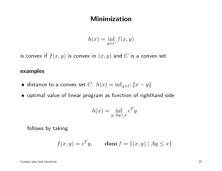
Minimization
h(x) = inf f (x, y)
yC

is convex if f (x, y) is convex in (x, y) and C is a convex set examples distance to a convex set C: h(x) = inf yC x y optimal value of linear program as function of righthand side h(x) = follows by taking f (x, y) = cT y,
Convex sets and functions

y:Ayx

inf

cT y

dom f = {(x, y) | Ay x}
19

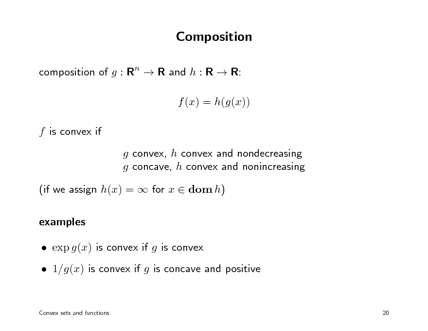
Composition
composition of g : Rn R and h : R R: f (x) = h(g(x)) f is convex if g convex, h convex and nondecreasing g concave, h convex and nonincreasing (if we assign h(x) = for x dom h) examples exp g(x) is convex if g is convex 1/g(x) is convex if g is concave and positive
Convex sets and functions 20

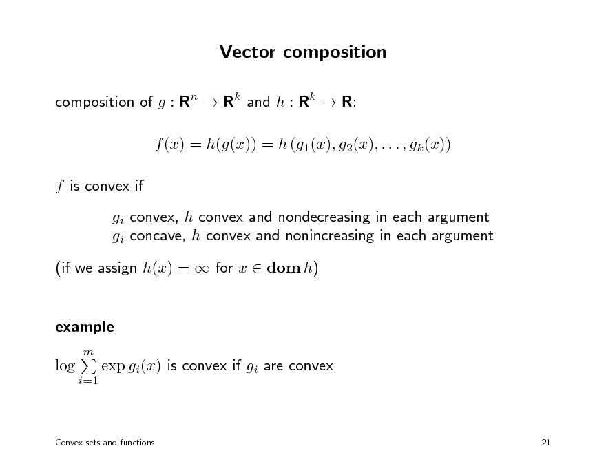
Vector composition
composition of g : Rn Rk and h : Rk R: f (x) = h(g(x)) = h (g1(x), g2(x), . . . , gk (x)) f is convex if gi convex, h convex and nondecreasing in each argument gi concave, h convex and nonincreasing in each argument (if we assign h(x) = for x dom h) example
m

log
i=1

exp gi(x) is convex if gi are convex

Convex sets and functions

21

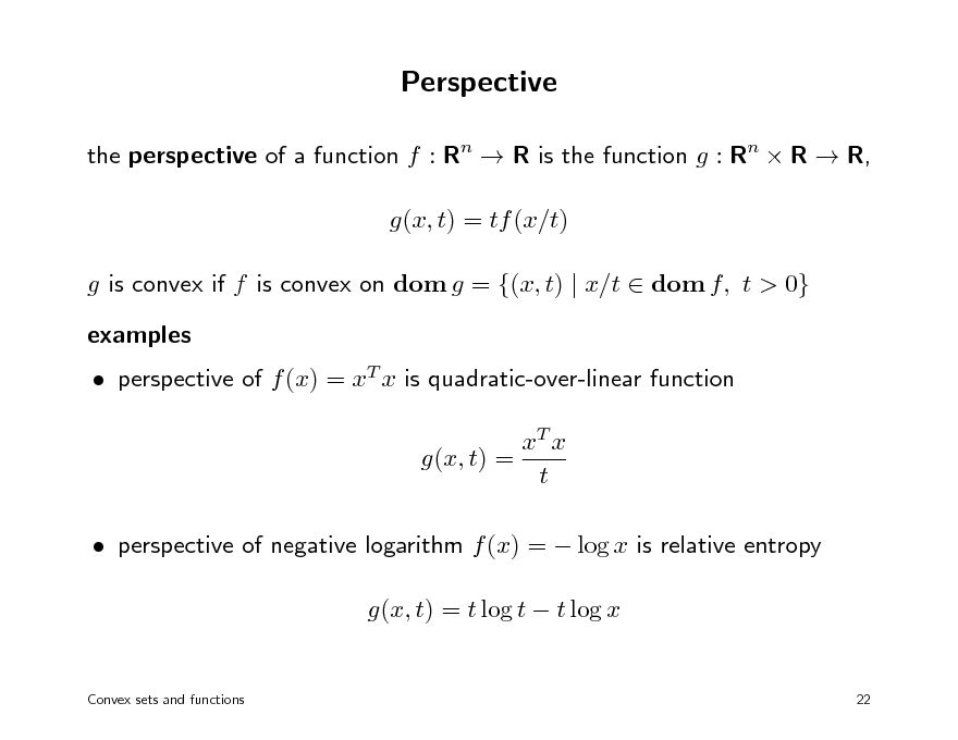
Perspective
the perspective of a function f : Rn R is the function g : Rn R R, g(x, t) = tf (x/t) g is convex if f is convex on dom g = {(x, t) | x/t dom f, t > 0} examples perspective of f (x) = xT x is quadratic-over-linear function xT x g(x, t) = t perspective of negative logarithm f (x) = log x is relative entropy g(x, t) = t log t t log x
Convex sets and functions 22

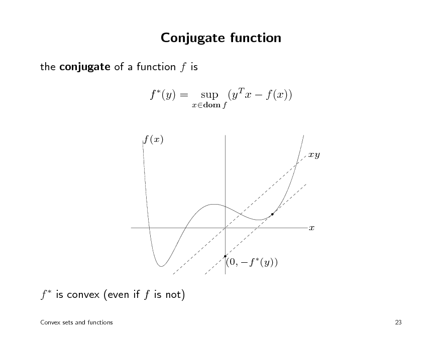
Conjugate function
the conjugate of a function f is f (y) =
xdom f

sup (y T x f (x))

f (x) xy

x (0, f (y))

f is convex (even if f is not)
Convex sets and functions 23

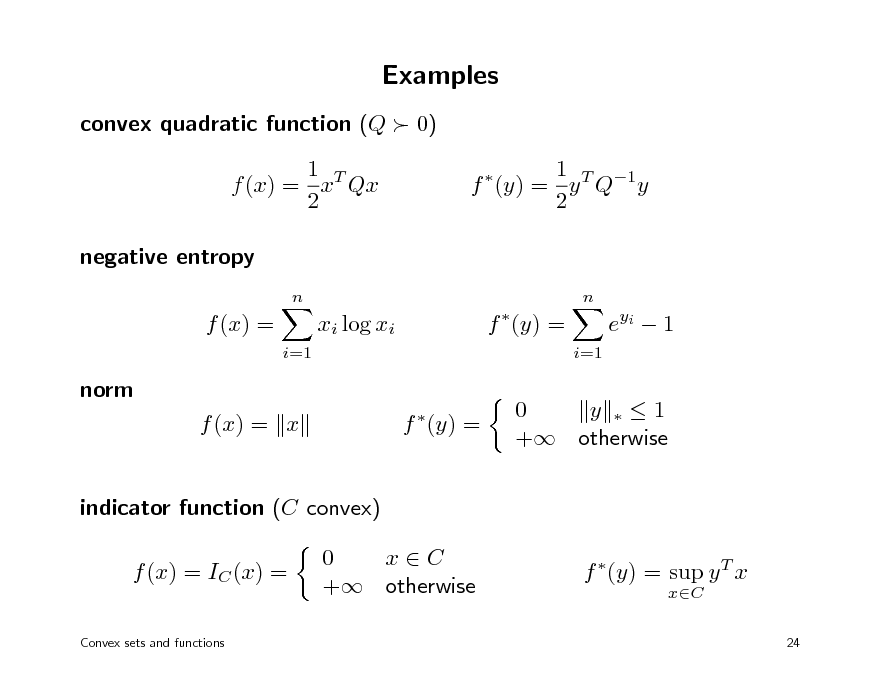
Examples
convex quadratic function (Q 0) 1 T f (x) = x Qx 2 negative entropy
n n

1 T 1 f (y) = y Q y 2

f (x) =
i=1

xi log xi

f (y) =
i=1

e yi 1

norm f (x) = x f (y) =

0 y 1 + otherwise

indicator function (C convex) f (x) = IC (x) =
Convex sets and functions

0 xC + otherwise

f (y) = sup y T x
xC
24

Convex optimization MLSS 2012

Convex optimization problems

linear programming quadratic programming geometric programming second-order cone programming semidenite programming

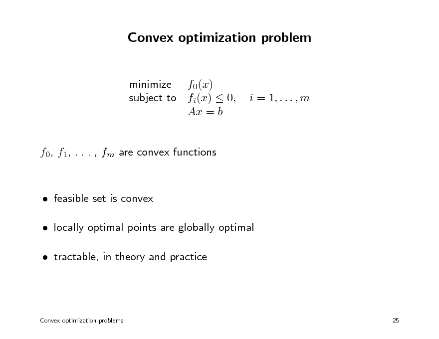
Convex optimization problem
minimize f0(x) subject to fi(x) 0, Ax = b

i = 1, . . . , m

f0, f1, . . . , fm are convex functions

feasible set is convex locally optimal points are globally optimal tractable, in theory and practice

Convex optimization problems

25

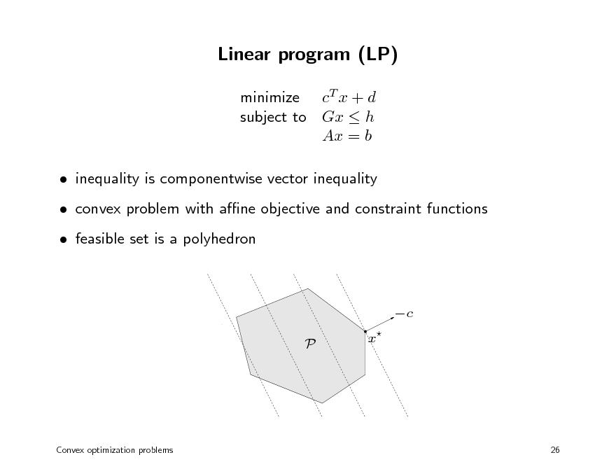
Linear program (LP)
minimize cT x + d subject to Gx h Ax = b inequality is componentwise vector inequality convex problem with ane objective and constraint functions feasible set is a polyhedron

c P x

Convex optimization problems

26

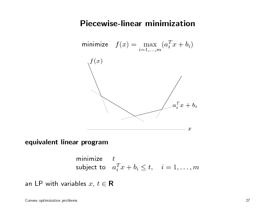
Piecewise-linear minimization
minimize f (x) = max (aT x + bi) i
i=1,...,m

f (x)

aT x + bi i

x

equivalent linear program minimize t subject to aT x + bi t, i an LP with variables x, t R
Convex optimization problems 27

i = 1, . . . , m

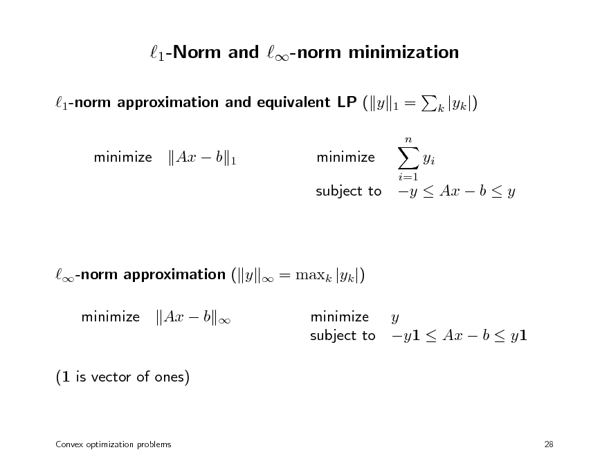
1-Norm and -norm minimization
1-norm approximation and equivalent LP ( y minimize Ax b minimize
i=1 1

=
n

k |yk |)

1

yi

subject to y Ax b y

-norm approximation ( y minimize Ax b

= maxk |yk |) minimize y subject to y1 Ax b y1

(1 is vector of ones)

Convex optimization problems

28

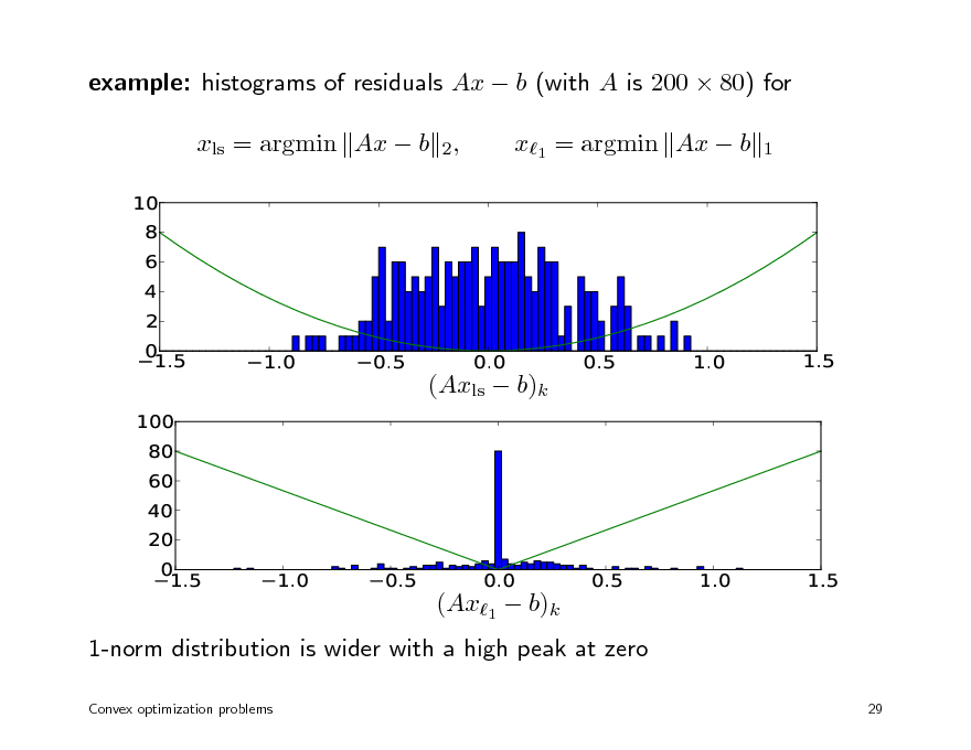
example: histograms of residuals Ax b (with A is 200 80) for xls = argmin Ax b 2,
10 8 6 4 2 0 1.5 1.0 0.5 0.0 0.5 1.0 1.5

x1 = argmin Ax b

1

(Axls b)k
100 80 60 40 20 0 1.5 1.0 0.5 0.0 0.5 1.0 1.5

(Ax1 b)k 1-norm distribution is wider with a high peak at zero
Convex optimization problems 29

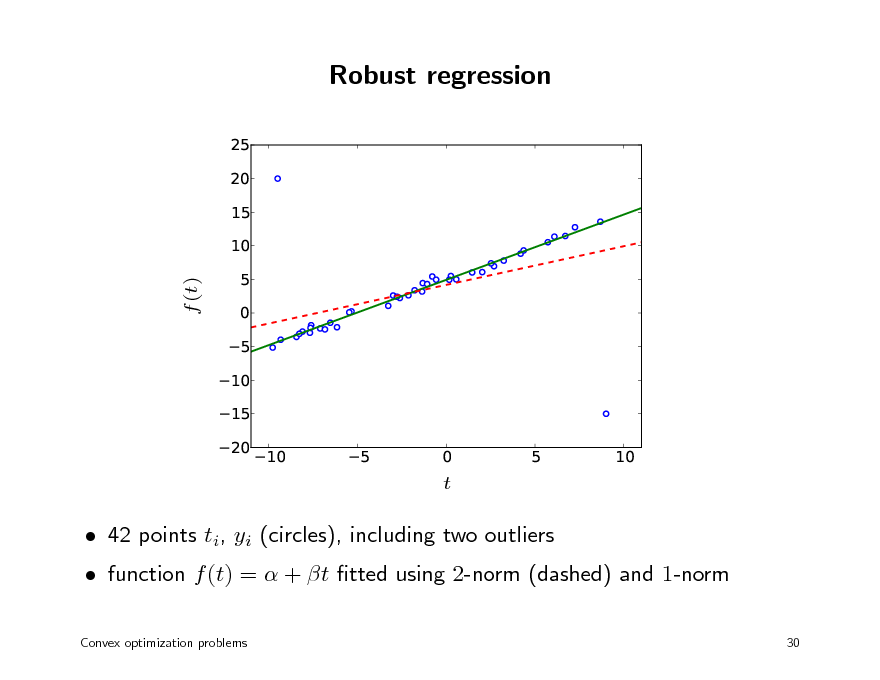
Robust regression
25 20 15 10 5 0 5 10 15 20 10

f (t)

5

0 t

5

10

function f (t) = + t tted using 2-norm (dashed) and 1-norm
Convex optimization problems 30

42 points ti, yi (circles), including two outliers

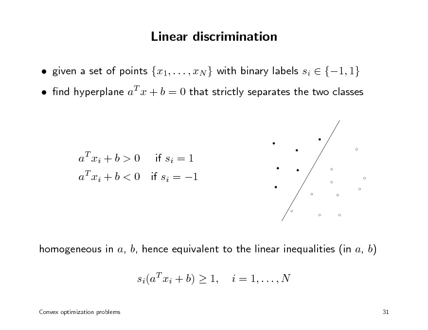
Linear discrimination
given a set of points {x1, . . . , xN } with binary labels si {1, 1} nd hyperplane aT x + b = 0 that strictly separates the two classes

a T xi + b > 0

if si = 1

aT xi + b < 0 if si = 1

homogeneous in a, b, hence equivalent to the linear inequalities (in a, b) si(aT xi + b) 1,
Convex optimization problems

i = 1, . . . , N
31

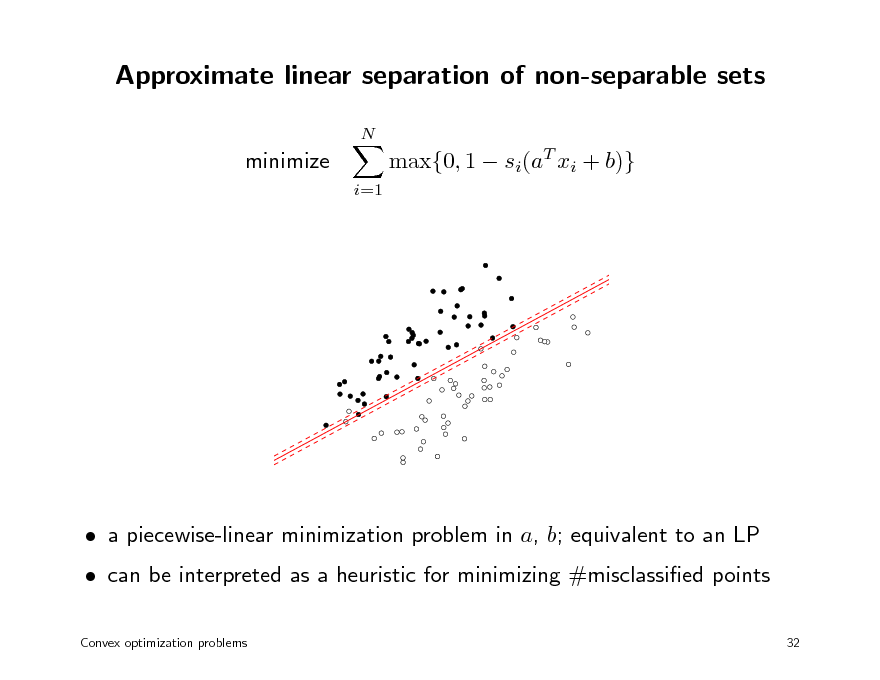
Approximate linear separation of non-separable sets
N

minimize
i=1

max{0, 1 si(aT xi + b)}

can be interpreted as a heuristic for minimizing #misclassied points
Convex optimization problems 32

a piecewise-linear minimization problem in a, b; equivalent to an LP

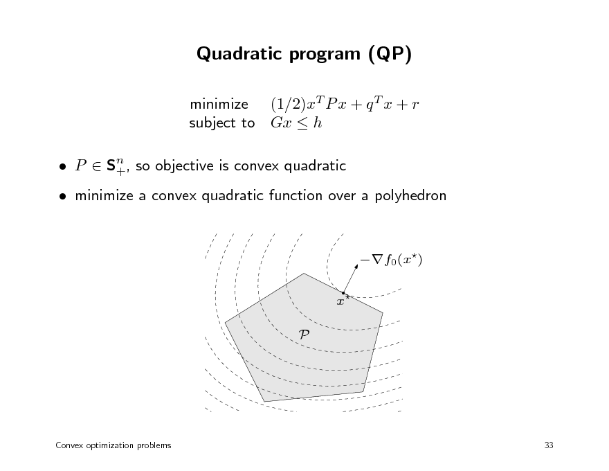
Quadratic program (QP)
minimize (1/2)xT P x + q T x + r subject to Gx h
n P S+, so objective is convex quadratic

minimize a convex quadratic function over a polyhedron
f0(x) x P

Convex optimization problems

33

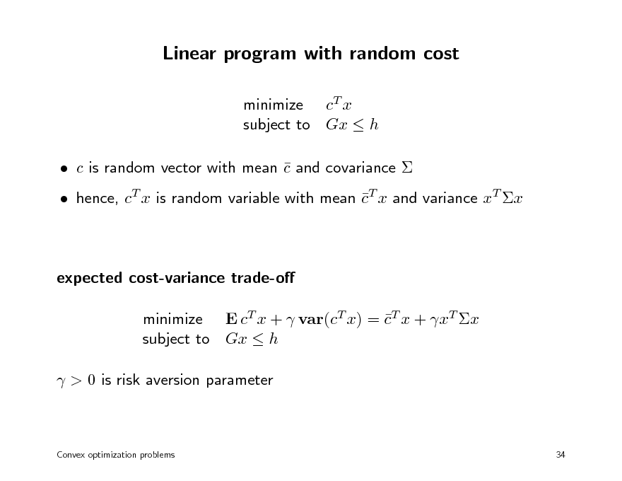
Linear program with random cost
minimize cT x subject to Gx h c is random vector with mean c and covariance hence, cT x is random variable with mean cT x and variance xT x

expected cost-variance trade-o minimize E cT x + var(cT x) = cT x + xT x subject to Gx h > 0 is risk aversion parameter

Convex optimization problems

34

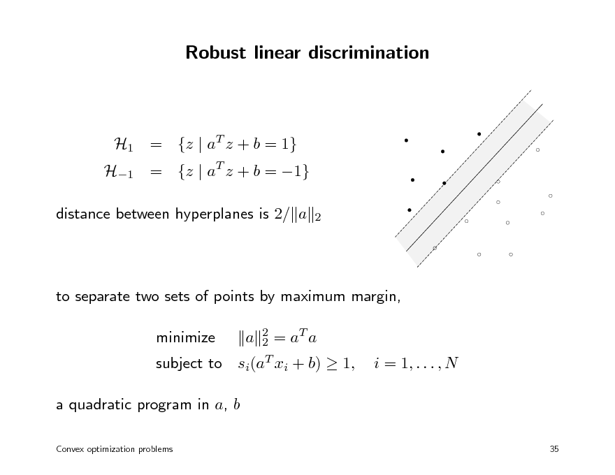
Robust linear discrimination

H1 = {z | aT z + b = 1} distance between hyperplanes is 2/ a
2

H1 = {z | aT z + b = 1}

to separate two sets of points by maximum margin, minimize subject to
2 T 2 =a a si(aT xi + b)

a

1,

i = 1, . . . , N

a quadratic program in a, b
Convex optimization problems 35

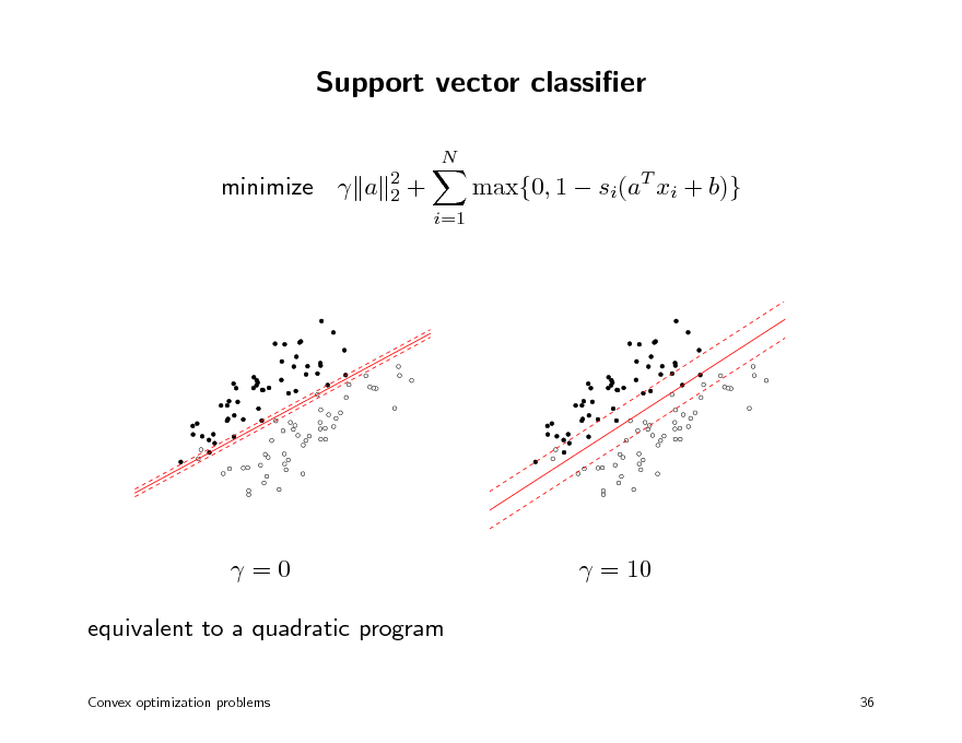
Support vector classier
N 2 2

minimize a

+
i=1

max{0, 1 si(aT xi + b)}

=0 equivalent to a quadratic program
Convex optimization problems

= 10

36

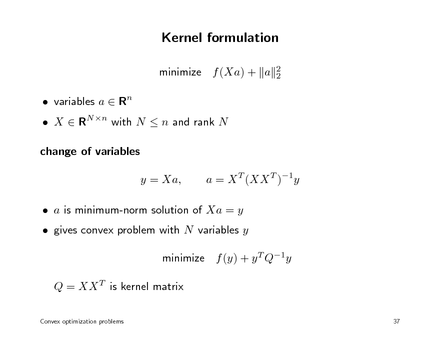
Kernel formulation
minimize f (Xa) + a variables a Rn
2 2

X RN n with N n and rank N change of variables y = Xa, a = X T (XX T )1y

a is minimum-norm solution of Xa = y gives convex problem with N variables y minimize f (y) + y T Q1y Q = XX T is kernel matrix
Convex optimization problems 37

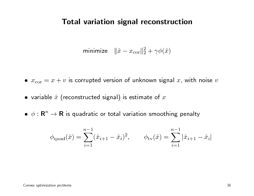
Total variation signal reconstruction

minimize

x xcor

2 2

+ () x

xcor = x + v is corrupted version of unknown signal x, with noise v variable x (reconstructed signal) is estimate of x : Rn R is quadratic or total variation smoothing penalty
n1 n1

quad() = x
i=1

(i+1 xi)2, x

tv () = x
i=1

|i+1 xi| x

Convex optimization problems

38

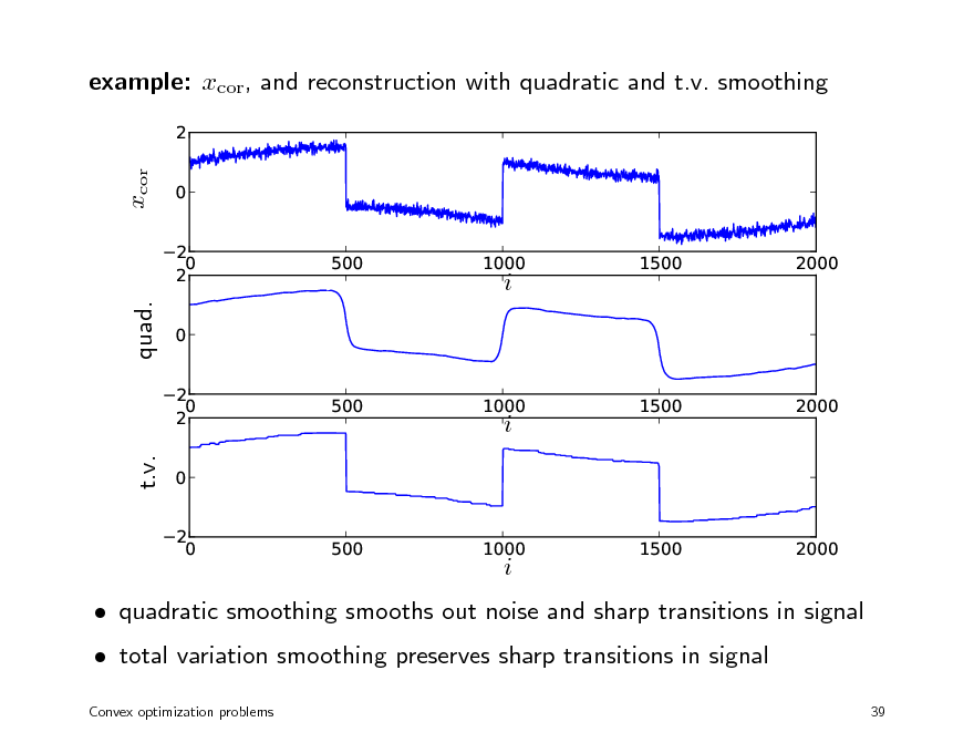
example: xcor, and reconstruction with quadratic and t.v. smoothing
2

xcor

0 2 0 2 0 2 0 2 0 2 0 500 1000 1500 2000

500

1000

i

1500

2000

quad.

500

1000

i

1500

2000

t.v.

i

quadratic smoothing smooths out noise and sharp transitions in signal total variation smoothing preserves sharp transitions in signal
Convex optimization problems 39

Geometric programming
posynomial function
K

f (x) =
k=1

ck x1 1k x2 2k xank , n

a

a

dom f = Rn ++

with ck > 0 geometric program (GP) minimize f0(x) subject to fi(x) 1, with fi posynomial

i = 1, . . . , m

Convex optimization problems

40

Geometric program in convex form
change variables to yi = log xi, and take logarithm of cost, constraints

geometric program in convex form:
K

minimize

log
k=1 K

exp(aT y + b0k ) 0k exp(aT y + bik ) ik
k=1

subject to log bik = log cik

0,

i = 1, . . . , m

Convex optimization problems

41

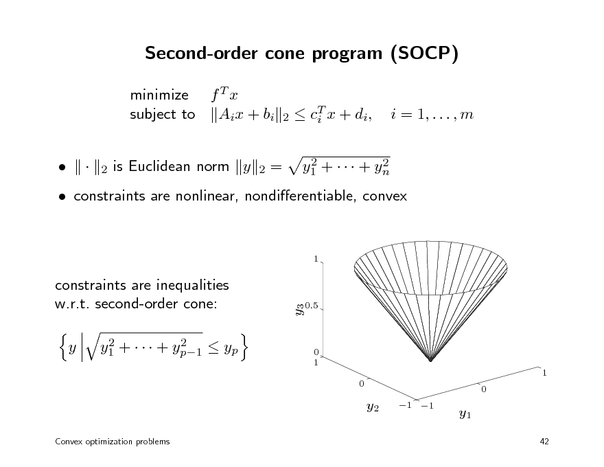
Second-order cone program (SOCP)
minimize f T x subject to Aix + bi is Euclidean norm y =
T c i x + di , 2 2 y1 + + yn

2

i = 1, . . . , m

2

2

constraints are nonlinear, nondierentiable, convex
1

y

2 2 y1 + + yp1 yp

y3

constraints are inequalities w.r.t. second-order cone:

0.5

0 1 1 0 0

y2
Convex optimization problems

1 1

y1
42

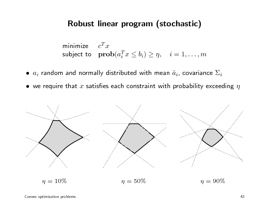
Robust linear program (stochastic)
minimize cT x subject to prob(aT x bi) , i

i = 1, . . . , m

ai random and normally distributed with mean ai, covariance i we require that x satises each constraint with probability exceeding

= 10%
Convex optimization problems

= 50%

= 90%
43

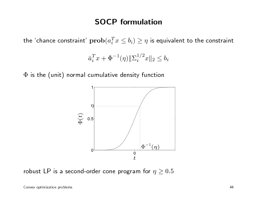
SOCP formulation
the chance constraint prob(aT x bi) is equivalent to the constraint i aT x + 1() i x i
1/2 2

bi

is the (unit) normal cumulative density function
1

(t)
0.5

0

1()
0

t

robust LP is a second-order cone program for 0.5
Convex optimization problems 44

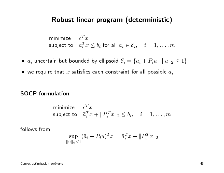
Robust linear program (deterministic)
minimize cT x subject to aT x bi for all ai Ei, i

i = 1, . . . , m
2

ai uncertain but bounded by ellipsoid Ei = {i + Piu | u a

1}

we require that x satises each constraint for all possible ai SOCP formulation minimize cT x subject to aT x + PiT x i follows from
u 2 1

2

bi ,

i = 1, . . . , m

sup (i + Piu)T x = aT x + PiT x a i

2

Convex optimization problems

45

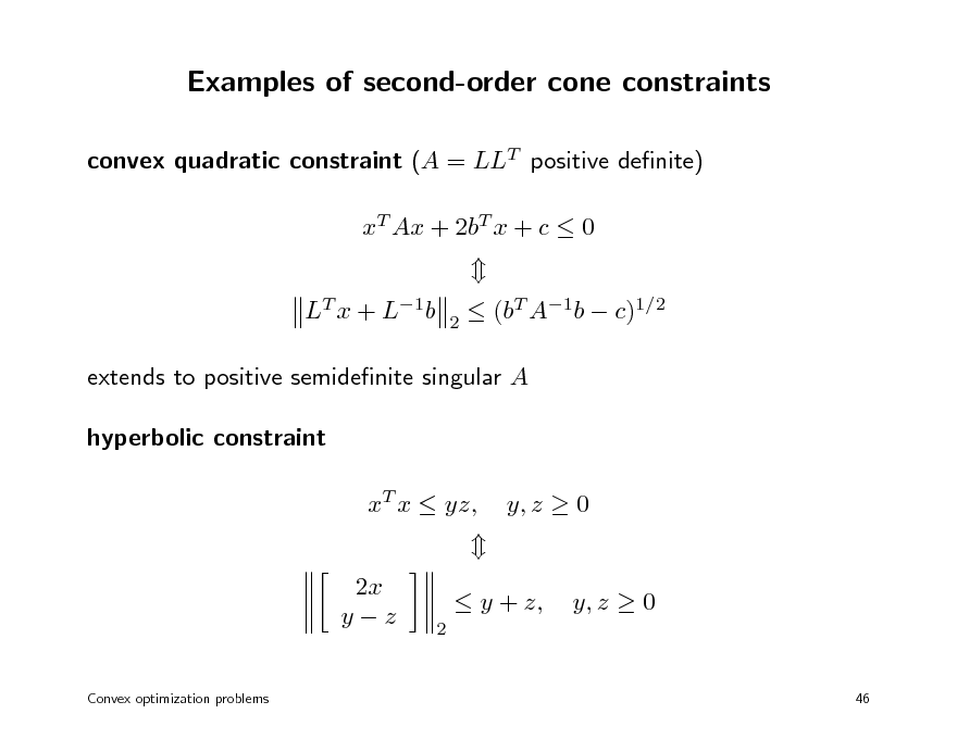
Examples of second-order cone constraints
convex quadratic constraint (A = LLT positive denite) xT Ax + 2bT x + c 0 LT x + L1b
2

(bT A1b c)1/2

extends to positive semidenite singular A hyperbolic constraint xT x yz, 2x yz
Convex optimization problems

y, z 0 y, z 0
46

2

y + z,

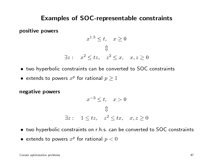
Examples of SOC-representable constraints
positive powers x1.5 t, z : x2 tz, x0 x, z 0

z 2 x,

extends to powers xp for rational p 1 negative powers x3 t, z : 1 tz,

two hyperbolic constraints can be converted to SOC constraints

x>0 x, z 0

z 2 tx,

extends to powers xp for rational p < 0
Convex optimization problems

two hyperbolic constraints on r.h.s. can be converted to SOC constraints

47

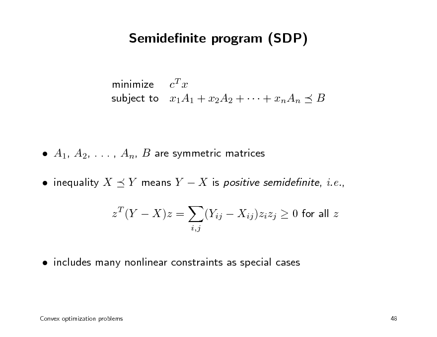
Semidenite program (SDP)
minimize cT x subject to x1A1 + x2A2 + + xnAn

B

A1, A2, . . . , An, B are symmetric matrices inequality X Y means Y X is positive semidenite, i.e.,
i,j

z T (Y X)z =

(Yij Xij )zizj 0 for all z

includes many nonlinear constraints as special cases

Convex optimization problems

48

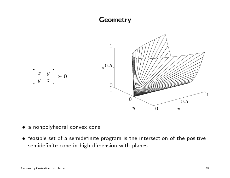
Geometry

1

x y y z

0
0 1 0 y 1 0 x 0.5 1

a nonpolyhedral convex cone feasible set of a semidenite program is the intersection of the positive semidenite cone in high dimension with planes

Convex optimization problems

z

0.5

49

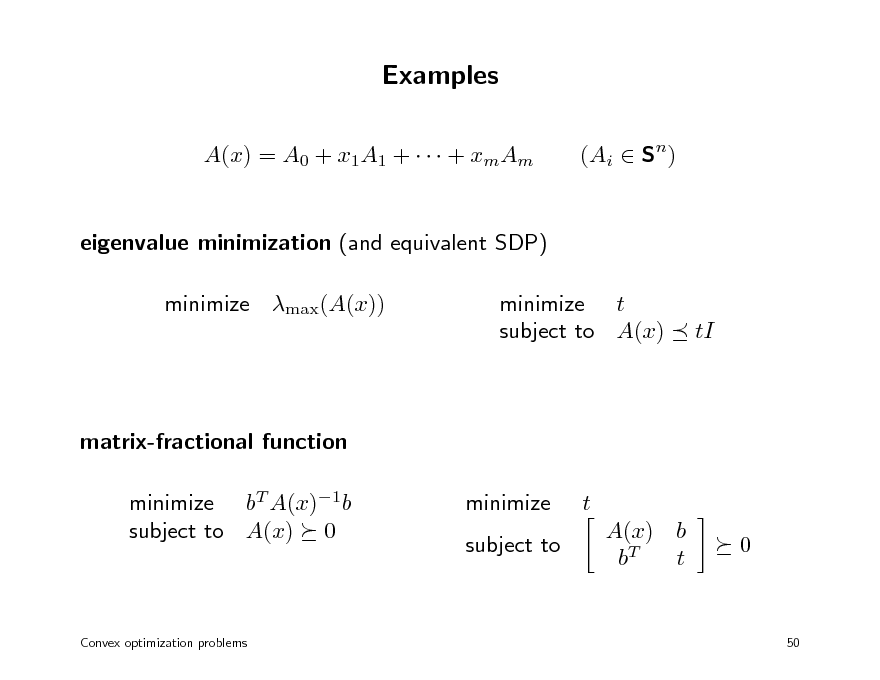
Examples
A(x) = A0 + x1A1 + + xmAm eigenvalue minimization (and equivalent SDP) minimize max(A(x)) minimize t subject to A(x) (Ai Sn)

tI

matrix-fractional function minimize bT A(x)1b subject to A(x) 0 minimize subject to t A(x) b bT t 0

Convex optimization problems

50

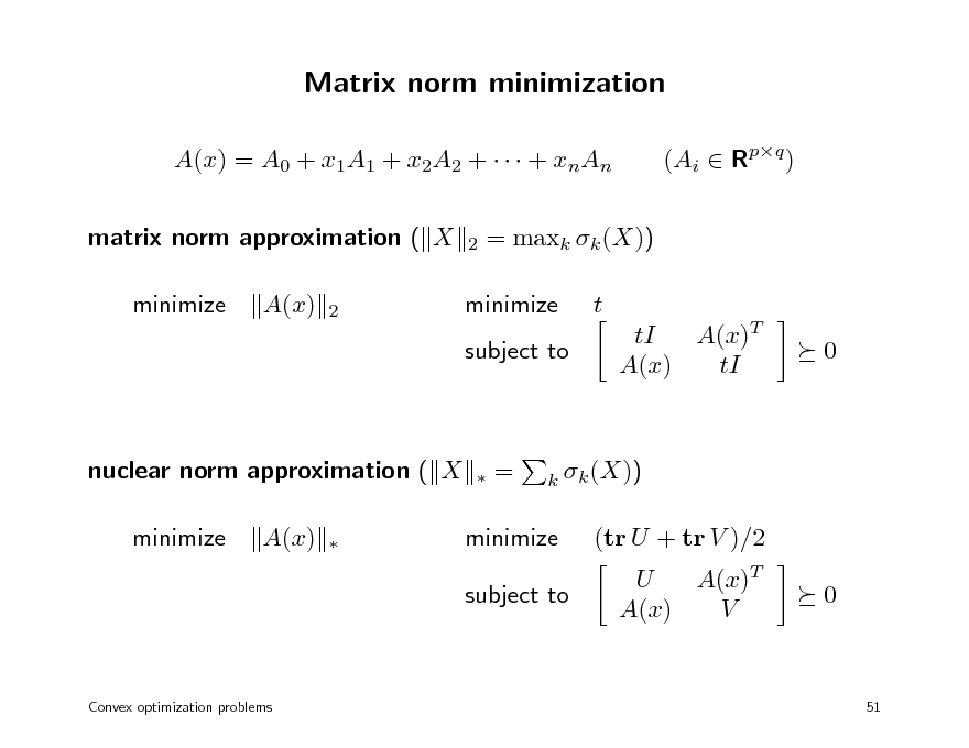
Matrix norm minimization
A(x) = A0 + x1A1 + x2A2 + + xnAn matrix norm approximation ( X minimize A(x)
2 2

(Ai Rpq )

= maxk k (X)) t tI A(x)T A(x) tI 0

minimize subject to

nuclear norm approximation ( X minimize A(x)

=

k k (X))

minimize subject to

(tr U + tr V )/2 U A(x)T A(x) V 0

Convex optimization problems

51

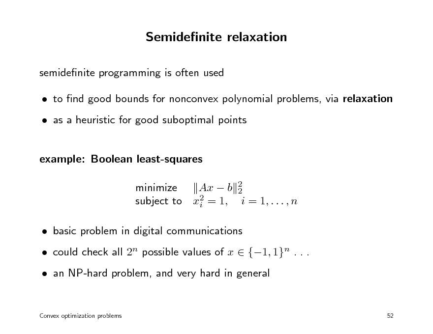
Semidenite relaxation
semidenite programming is often used to nd good bounds for nonconvex polynomial problems, via relaxation as a heuristic for good suboptimal points example: Boolean least-squares minimize Ax b 2 2 2 subject to xi = 1, i = 1, . . . , n basic problem in digital communications could check all 2n possible values of x {1, 1}n . . . an NP-hard problem, and very hard in general
Convex optimization problems 52

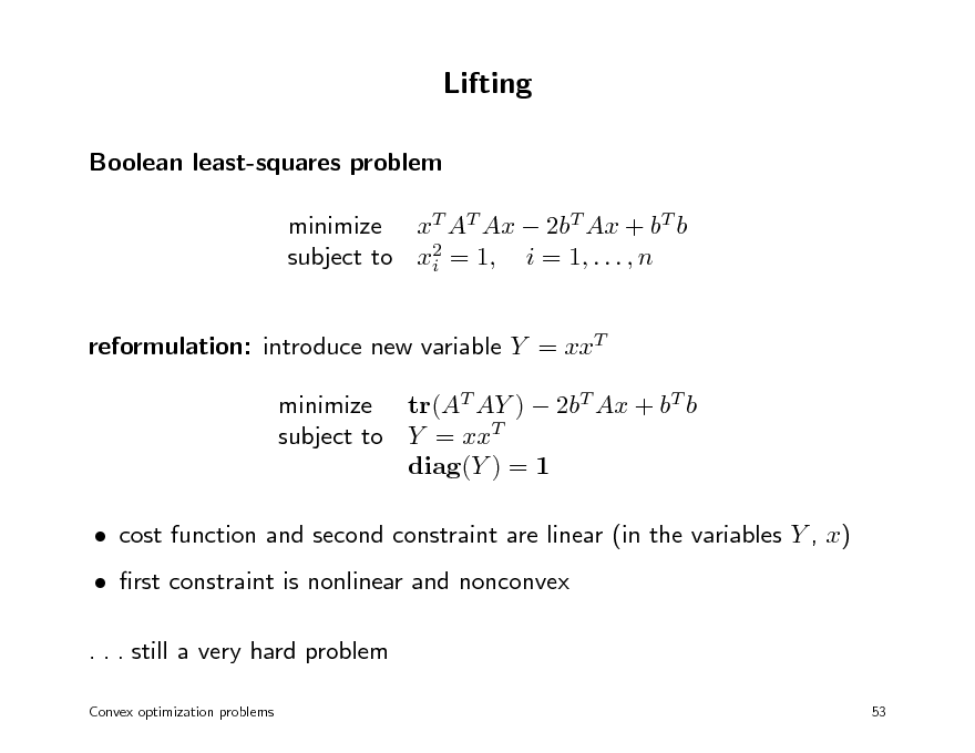
Lifting
Boolean least-squares problem minimize xT AT Ax 2bT Ax + bT b subject to x2 = 1, i = 1, . . . , n i reformulation: introduce new variable Y = xxT minimize tr(AT AY ) 2bT Ax + bT b subject to Y = xxT diag(Y ) = 1 cost function and second constraint are linear (in the variables Y , x) rst constraint is nonlinear and nonconvex . . . still a very hard problem
Convex optimization problems 53

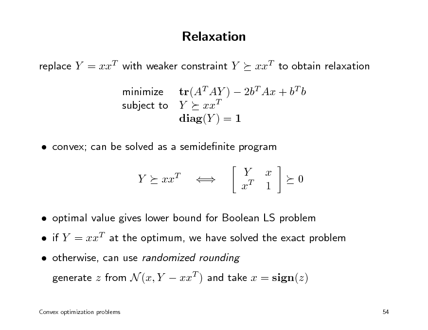
Relaxation
replace Y = xxT with weaker constraint Y xxT to obtain relaxation

minimize tr(AT AY ) 2bT Ax + bT b subject to Y xxT diag(Y ) = 1 convex; can be solved as a semidenite program Y xxT Y xT x 1 0

if Y = xxT at the optimum, we have solved the exact problem otherwise, can use randomized rounding generate z from N (x, Y xxT ) and take x = sign(z)
54

optimal value gives lower bound for Boolean LS problem

Convex optimization problems

Example
0.5

0.4

SDP bound

LS solution

frequency

0.3

0.2

0.1

0

1

1.2
2 /(SDP

Ax b

bound)

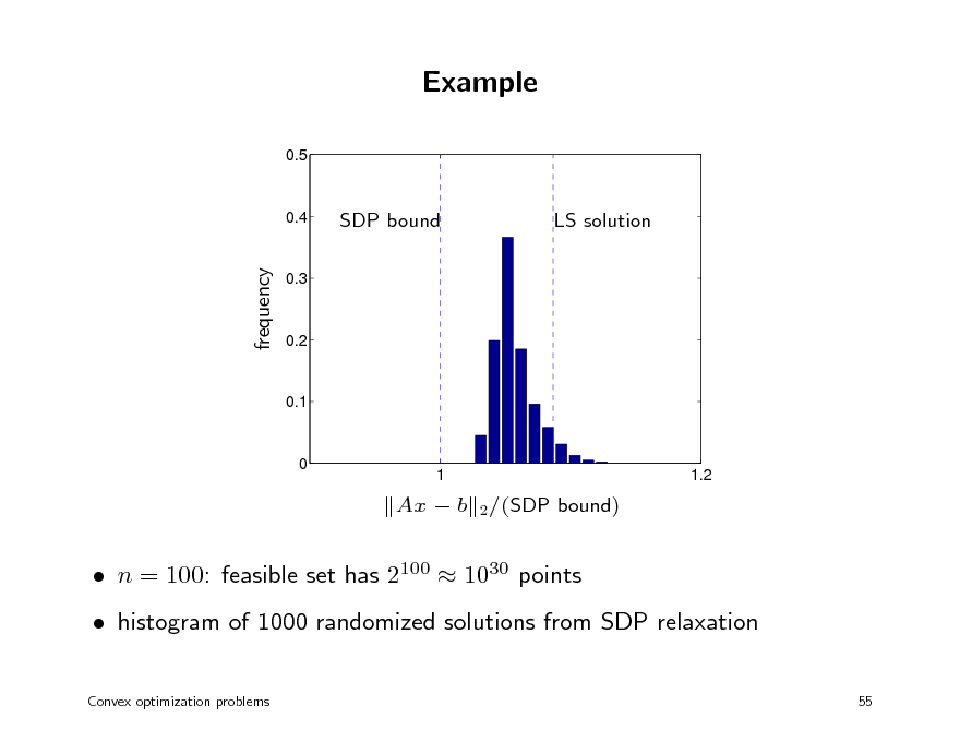
n = 100: feasible set has 2100 1030 points histogram of 1000 randomized solutions from SDP relaxation
Convex optimization problems 55

Overview

1. Basic theory and convex modeling convex sets and functions common problem classes and applications 2. Interior-point methods for conic optimization conic optimization barrier methods symmetric primal-dual methods 3. First-order methods (proximal) gradient algorithms dual techniques and multiplier methods

Convex optimization MLSS 2012

Conic optimization

denitions and examples modeling duality

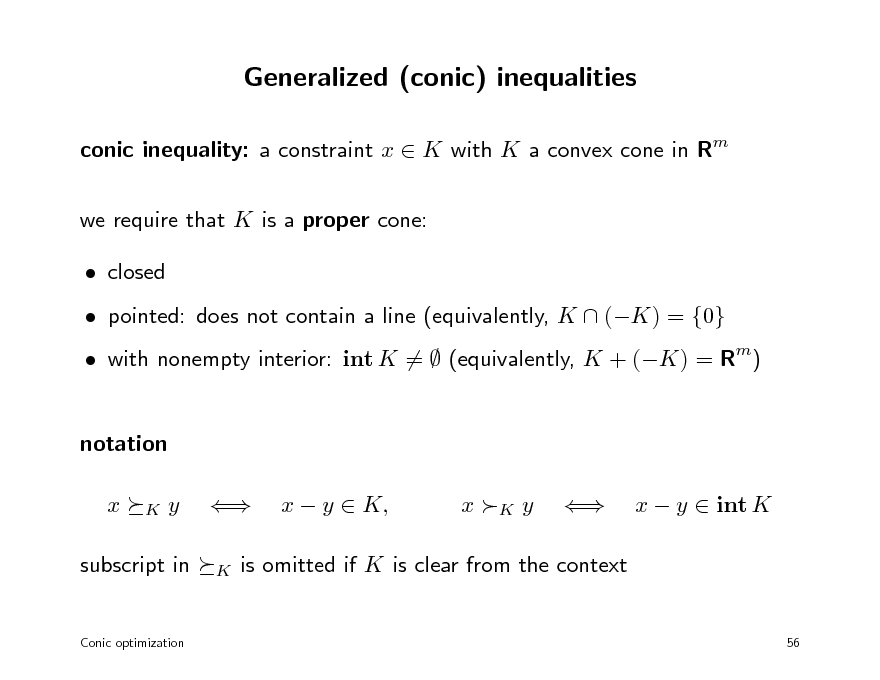
Generalized (conic) inequalities
conic inequality: a constraint x K with K a convex cone in Rm we require that K is a proper cone: closed pointed: does not contain a line (equivalently, K (K) = {0} with nonempty interior: int K = (equivalently, K + (K) = Rm)

notation x
K

y

K

x y K,

x K y

x y int K

subscript in

is omitted if K is clear from the context

Conic optimization

56

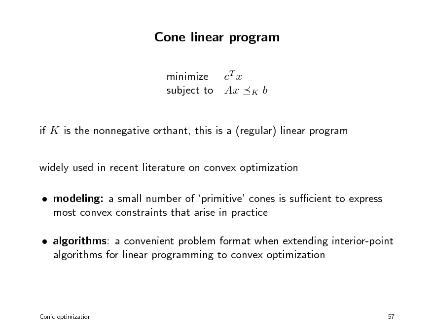
Cone linear program
minimize cT x subject to Ax

K

b

if K is the nonnegative orthant, this is a (regular) linear program widely used in recent literature on convex optimization modeling: a small number of primitive cones is sucient to express most convex constraints that arise in practice algorithms: a convenient problem format when extending interior-point algorithms for linear programming to convex optimization

Conic optimization

57

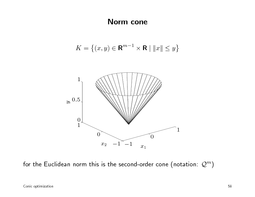
Norm cone
K = (x, y) Rm1 R | x y

1

y

0.5

0 1 0 x2 1 1 x1 0

1

for the Euclidean norm this is the second-order cone (notation: Qm)
Conic optimization 58

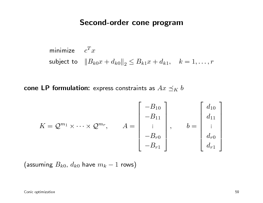
Second-order cone program
minimize subject to cT x Bk0x + dk0
2

Bk1x + dk1,

k = 1, . . . , r

cone LP formulation: express constraints as Ax B10 B11 . . Br0 Br1

K

b d10 d11 . . dr0 dr1

K = Q m1 Q mr ,

A=

,

b=

(assuming Bk0, dk0 have mk 1 rows)

Conic optimization

59

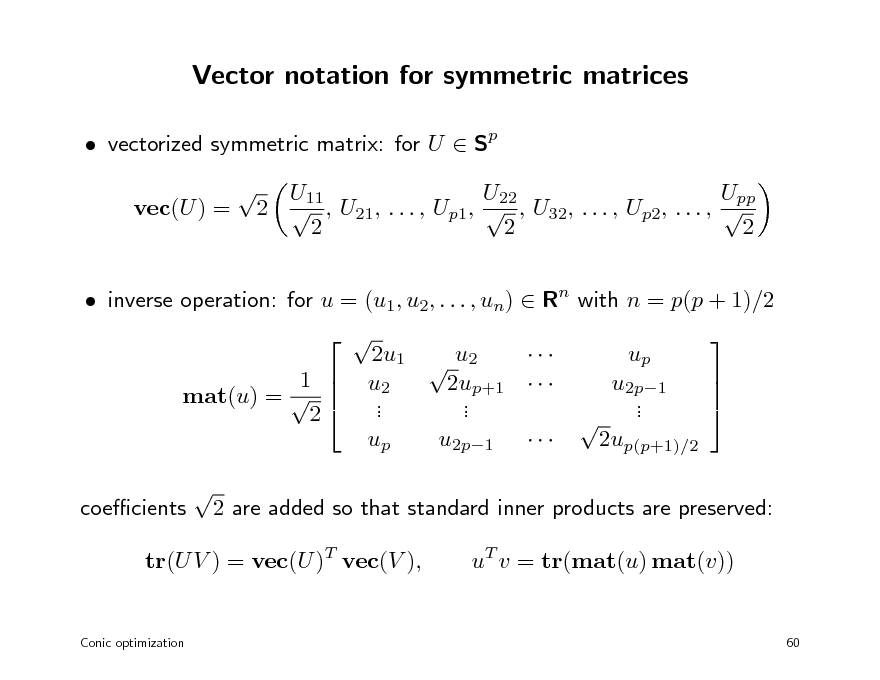
Vector notation for symmetric matrices
vectorized symmetric matrix: for U Sp vec(U ) = U11 U22 Upp 2 , U21, . . . , Up1, , U32, . . . , Up2, . . . , 2 2 2

inverse operation: for u = (u1, u2, . . . , un) Rn with n = p(p + 1)/2 1 mat(u) = 2 coecients 2u1 u2 u2 2up+1 . . . . up u2p1 up u2p1 . . 2up(p+1)/2

2 are added so that standard inner products are preserved: uT v = tr(mat(u) mat(v))

tr(U V ) = vec(U )T vec(V ),

Conic optimization

60

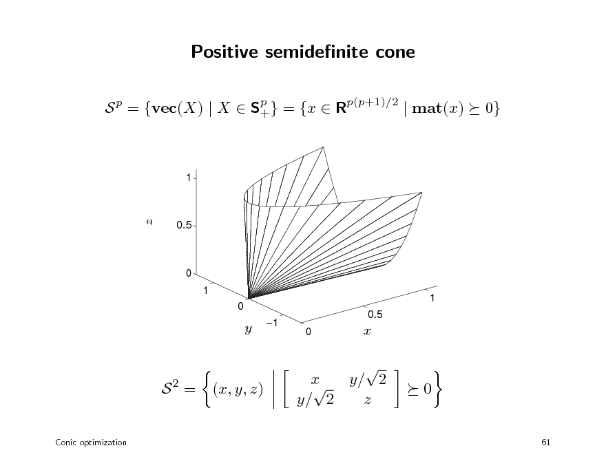
Positive semidenite cone
S p = {vec(X) | X Sp } = {x Rp(p+1)/2 | mat(x) + 0}

1

z

0.5

0 1 0 1

y

1

0.5 0

x

S2 =
Conic optimization

(x, y, z)

x y/ 2 y/ 2 z

0

61

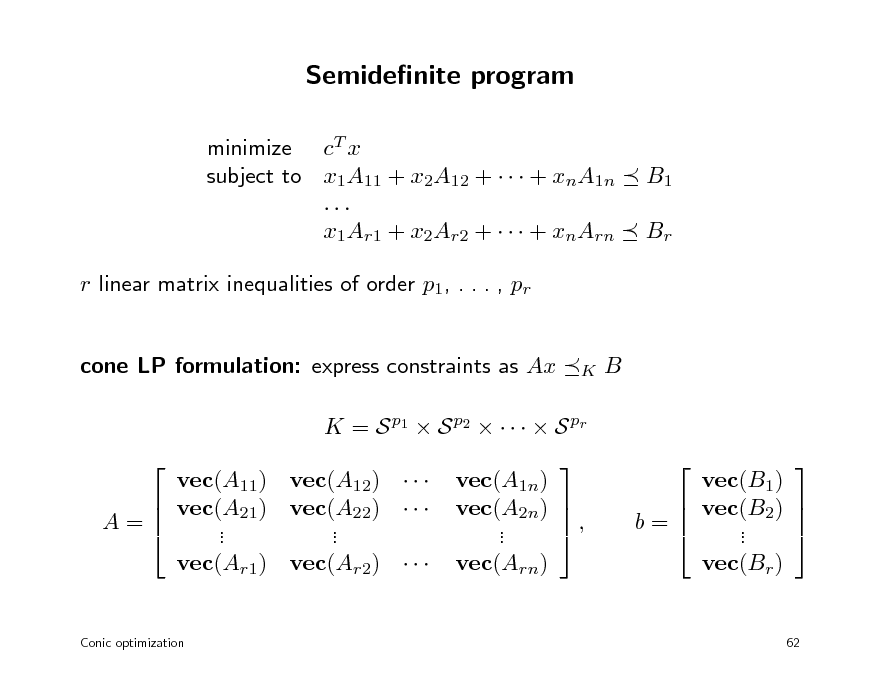
Semidenite program
minimize cT x subject to x1A11 + x2A12 + + xnA1n ... x1Ar1 + x2Ar2 + + xnArn r linear matrix inequalities of order p1, . . . , pr cone LP formulation: express constraints as Ax B

B1 Br

K

K = S p1 S p2 S pr vec(A11) vec(A12) vec(A21) vec(A22) A= . . . . vec(Ar1) vec(Ar2)
Conic optimization

vec(A1n) vec(A2n) , . . vec(Arn)

vec(B1) vec(B2) b= . . vec(Br )
62

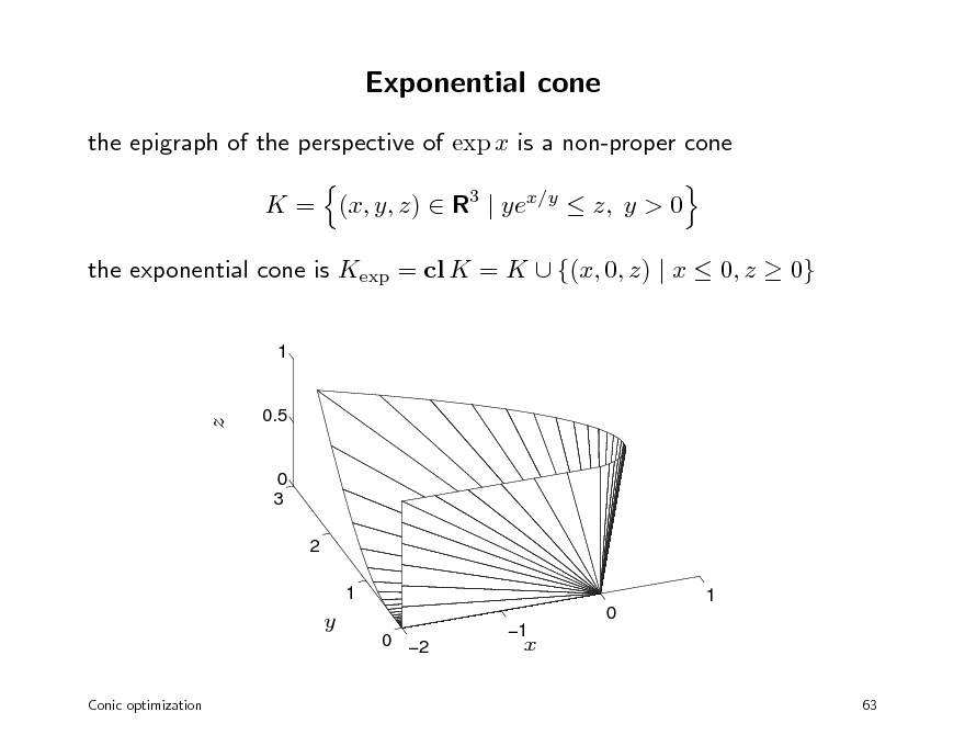
Exponential cone
the epigraph of the perspective of exp x is a non-proper cone K = (x, y, z) R3 | yex/y z, y > 0 the exponential cone is Kexp = cl K = K {(x, 0, z) | x 0, z 0}
1

z

0.5

0 3 2 1 1 0 0 2
Conic optimization

y

1

x
63

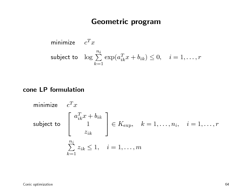
Geometric program
minimize cT x
ni k=1

subject to log

exp(aT x + bik ) 0, ik

i = 1, . . . , r

cone LP formulation cT x T aik x + bik Kexp, 1 subject to zik minimize
ni k=1

k = 1, . . . , ni,

i = 1, . . . , r

zik 1,

i = 1, . . . , m

Conic optimization

64

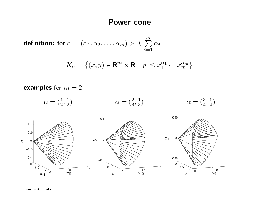
Power cone
m

denition: for = (1, 2, . . . , m) > 0,
i=1

i = 1

K = (x, y) Rm R | |y| x1 xmm + 1

examples for m = 2
1 = (1, 2) 2
0.5
0.4 0.2

1 = (2, 3) 3
0.5

3 1 = (4, 4)

y

0 0.2 0.4 0 0.5

y

0

y
0.5

0

0.5 0

0.5 0
1

x1

1 0

x2

0.5

1

0.5

x1

1 0

x2

0.5

x1

1 0

x2

0.5

1

Conic optimization

65

Outline

denition and examples modeling duality

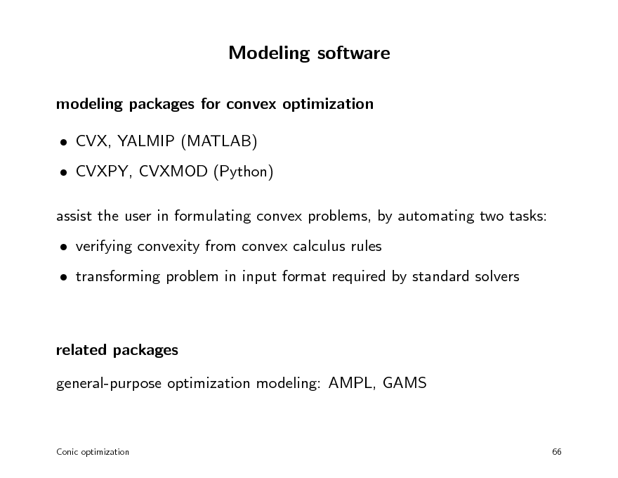
Modeling software
modeling packages for convex optimization CVX, YALMIP (MATLAB) CVXPY, CVXMOD (Python) assist the user in formulating convex problems, by automating two tasks: verifying convexity from convex calculus rules transforming problem in input format required by standard solvers

related packages general-purpose optimization modeling: AMPL, GAMS

Conic optimization

66

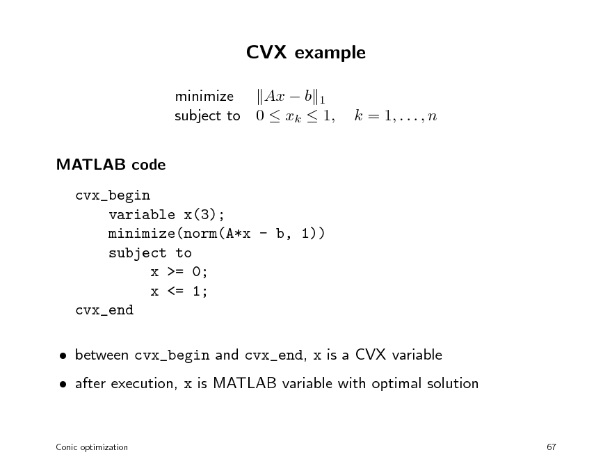
CVX example
minimize Ax b 1 subject to 0 xk 1, MATLAB code cvx_begin variable x(3); minimize(norm(A*x - b, 1)) subject to x >= 0; x <= 1; cvx_end between cvx_begin and cvx_end, x is a CVX variable after execution, x is MATLAB variable with optimal solution
Conic optimization 67

k = 1, . . . , n

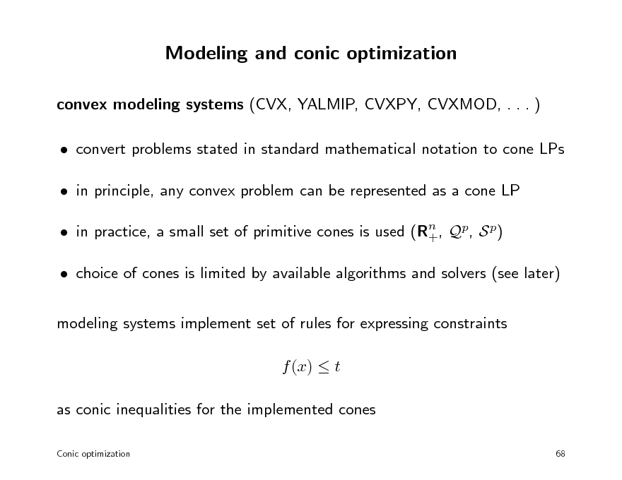
Modeling and conic optimization
convex modeling systems (CVX, YALMIP, CVXPY, CVXMOD, . . . ) convert problems stated in standard mathematical notation to cone LPs in principle, any convex problem can be represented as a cone LP in practice, a small set of primitive cones is used (Rn , Qp, S p) + choice of cones is limited by available algorithms and solvers (see later) modeling systems implement set of rules for expressing constraints f (x) t as conic inequalities for the implemented cones
Conic optimization 68

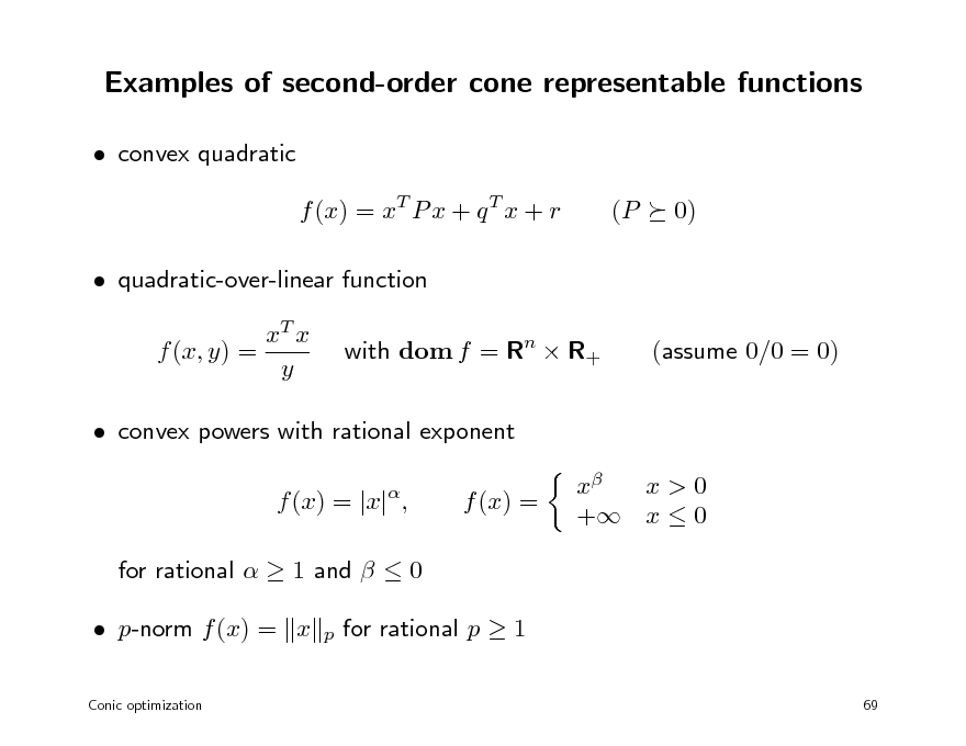
Examples of second-order cone representable functions
convex quadratic f (x) = xT P x + q T x + r quadratic-over-linear function xT x f (x, y) = y with dom f = Rn R+ (assume 0/0 = 0) (P 0)

convex powers with rational exponent f (x) = |x| , for rational 1 and 0 p-norm f (x) = x
Conic optimization

f (x) =

x x>0 + x 0

p

for rational p 1
69

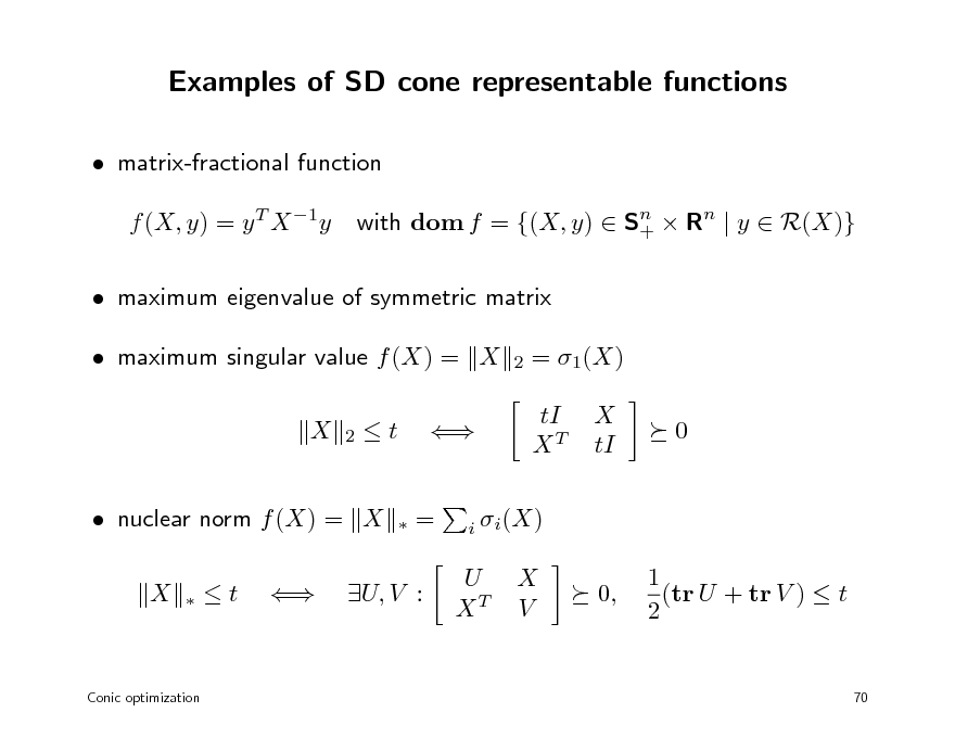
Examples of SD cone representable functions
matrix-fractional function f (X, y) = y T X 1y with dom f = {(X, y) Sn Rn | y R(X)} +

maximum eigenvalue of symmetric matrix maximum singular value f (X) = X X
2 2

= 1(X) tI XT X tI 0

t

=

nuclear norm f (X) = X X

i i (X)

t

U, V :

U XT

X V

0,

1 (tr U + tr V ) t 2

Conic optimization

70

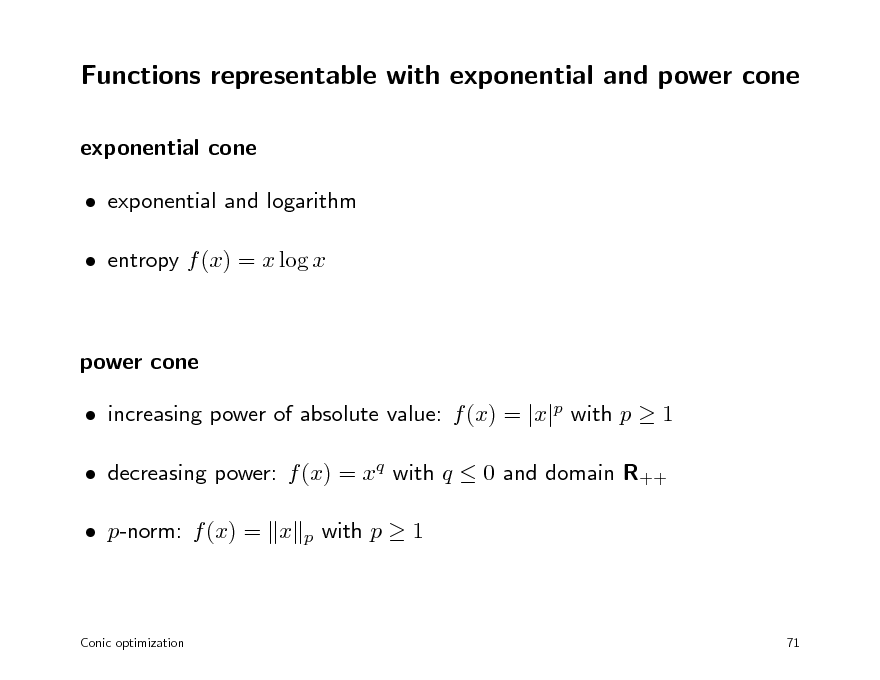
Functions representable with exponential and power cone
exponential cone exponential and logarithm entropy f (x) = x log x

power cone increasing power of absolute value: f (x) = |x|p with p 1 decreasing power: f (x) = xq with q 0 and domain R++ p-norm: f (x) = x
p

with p 1

Conic optimization

71

Outline

denition and examples modeling duality

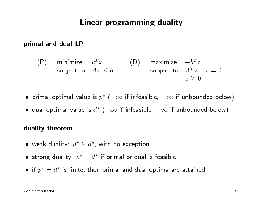
Linear programming duality
primal and dual LP (P) minimize cT x subject to Ax b (D) maximize bT z subject to AT z + c = 0 z0

primal optimal value is p (+ if infeasible, if unbounded below) dual optimal value is d ( if infeasible, + if unbounded below) duality theorem weak duality: p d, with no exception strong duality: p = d if primal or dual is feasible if p = d is nite, then primal and dual optima are attained
Conic optimization 72

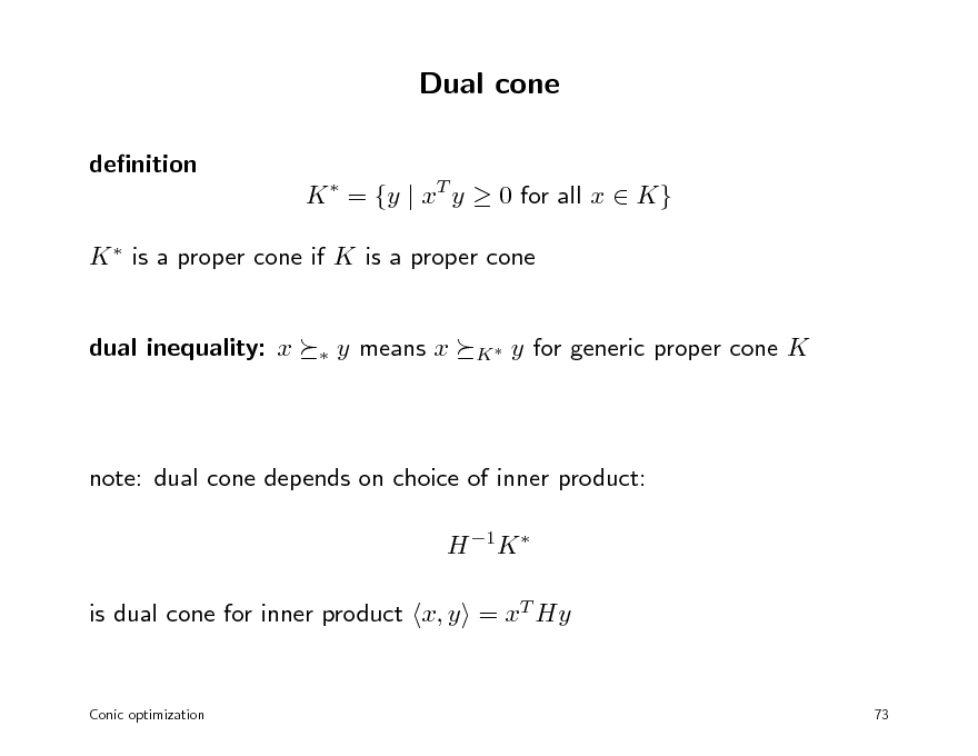
Dual cone
denition K = {y | xT y 0 for all x K} K is a proper cone if K is a proper cone

dual inequality: x

y means x

K

y for generic proper cone K

note: dual cone depends on choice of inner product: H 1K is dual cone for inner product x, y = xT Hy

Conic optimization

73

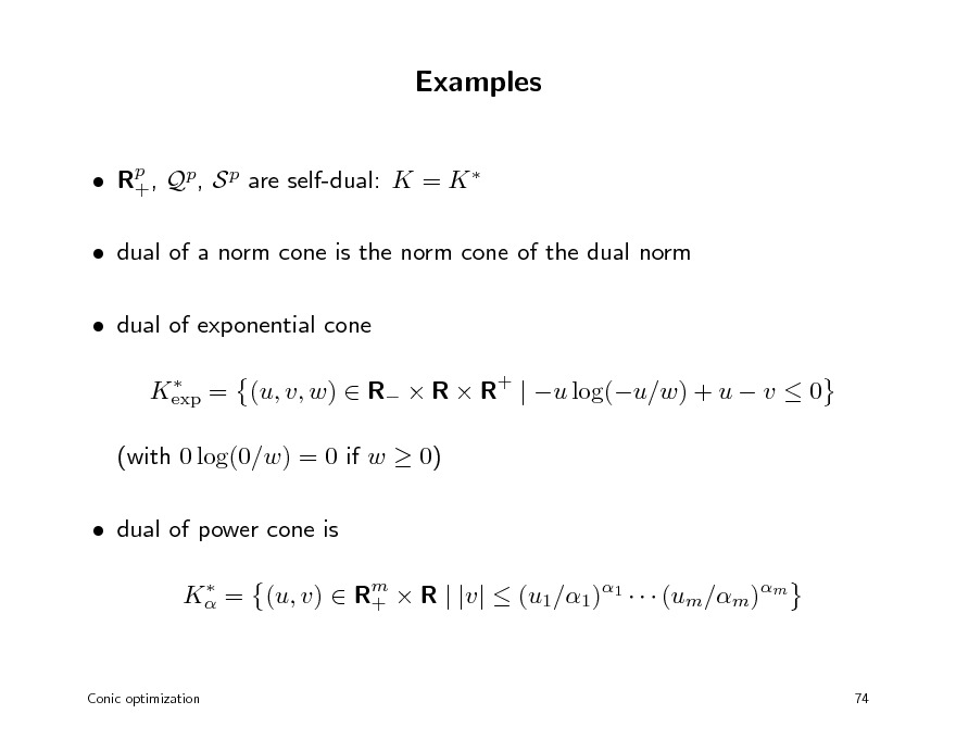
Examples
Rp , Qp, S p are self-dual: K = K + dual of a norm cone is the norm cone of the dual norm dual of exponential cone
Kexp = (u, v, w) R R R+ | u log(u/w) + u v 0

(with 0 log(0/w) = 0 if w 0) dual of power cone is
K = (u, v) Rm R | |v| (u1/1)1 (um/m)m +

Conic optimization

74

Primal and dual cone LP
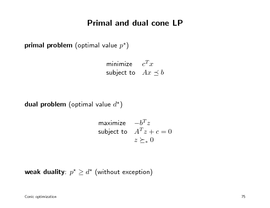
primal problem (optimal value p) minimize cT x subject to Ax

b

dual problem (optimal value d) maximize bT z subject to AT z + c = 0 z 0

weak duality: p d (without exception)
Conic optimization 75

Strong duality
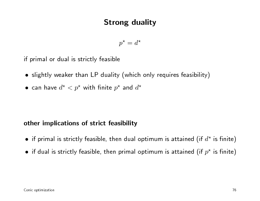
p = d if primal or dual is strictly feasible slightly weaker than LP duality (which only requires feasibility) can have d < p with nite p and d

other implications of strict feasibility if primal is strictly feasible, then dual optimum is attained (if d is nite) if dual is strictly feasible, then primal optimum is attained (if p is nite)

Conic optimization

76

Optimality conditions
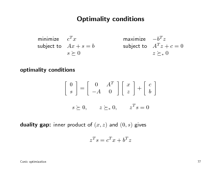
minimize cT x subject to Ax + s = b s 0 optimality conditions 0 s s = 0, 0 AT A 0 z

maximize bT z subject to AT z + c = 0 z 0

x z

+

c b

0,

zT s = 0

duality gap: inner product of (x, z) and (0, s) gives z T s = c T x + bT z

Conic optimization

77

Convex optimization MLSS 2012

Barrier methods

barrier method for linear programming normal barriers barrier method for conic optimization

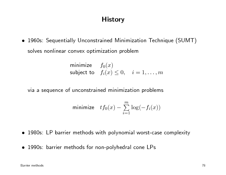
History
1960s: Sequentially Unconstrained Minimization Technique (SUMT) solves nonlinear convex optimization problem minimize f0(x) subject to fi(x) 0,

i = 1, . . . , m

via a sequence of unconstrained minimization problems
m

minimize tf0(x)

log(fi(x))
i=1

1980s: LP barrier methods with polynomial worst-case complexity 1990s: barrier methods for non-polyhedral cone LPs
Barrier methods 78

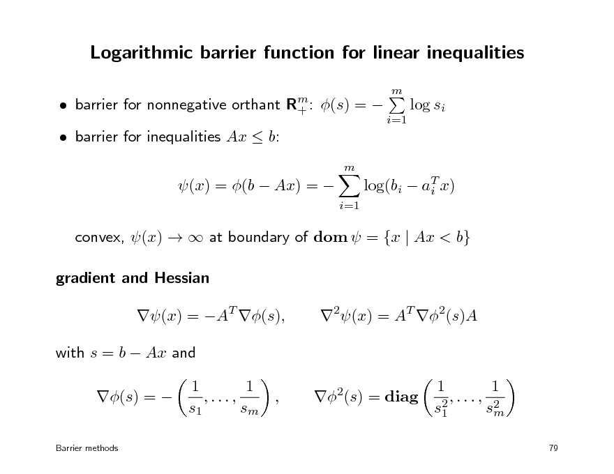
Logarithmic barrier function for linear inequalities
barrier for nonnegative orthant barrier for inequalities Ax b:
m

Rm : +

m

(s) =

log si
i=1

(x) = (b Ax) =

i=1

log(bi aT x) i

convex, (x) at boundary of dom = {x | Ax < b} gradient and Hessian (x) = AT (s), with s = b Ax and (s) =
Barrier methods

2(x) = AT 2(s)A

1 1 ,..., , s1 sm

2(s) = diag

1 1 ,..., 2 s2 sm 1
79

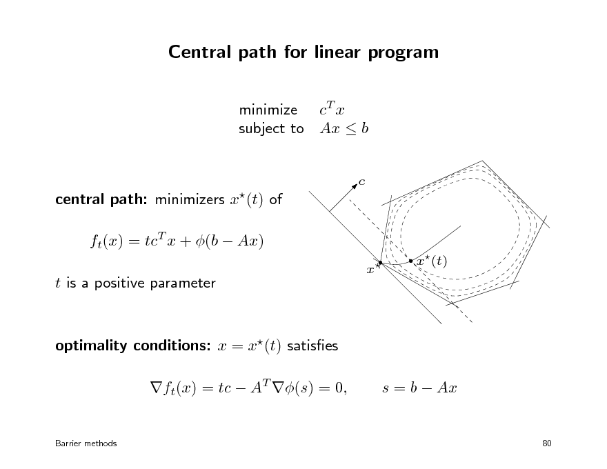
Central path for linear program
minimize cT x subject to Ax b
c

central path: minimizers x(t) of ft(x) = tcT x + (b Ax) t is a positive parameter
x

x(t)

optimality conditions: x = x(t) satises ft(x) = tc AT (s) = 0,
Barrier methods

s = b Ax
80

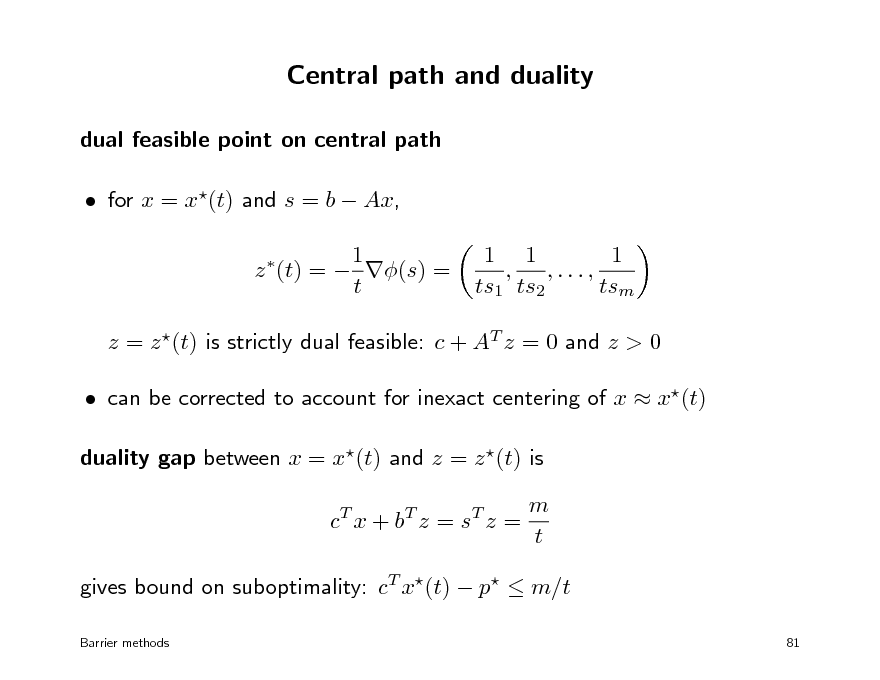
Central path and duality
dual feasible point on central path for x = x(t) and s = b Ax, 1 z (t) = (s) = t

1 1 1 , ,..., ts1 ts2 tsm

z = z (t) is strictly dual feasible: c + AT z = 0 and z > 0 can be corrected to account for inexact centering of x x(t) duality gap between x = x(t) and z = z (t) is c T x + bT z = s T z = m t

gives bound on suboptimality: cT x(t) p m/t
Barrier methods 81

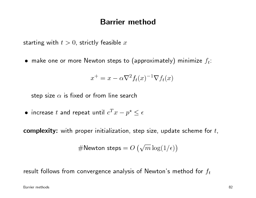
Barrier method
starting with t > 0, strictly feasible x make one or more Newton steps to (approximately) minimize ft: x+ = x 2ft(x)1ft(x) step size is xed or from line search increase t and repeat until cT x p complexity: with proper initialization, step size, update scheme for t, #Newton steps = O m log(1/)

result follows from convergence analysis of Newtons method for ft
Barrier methods 82

Outline

barrier method for linear programming normal barriers barrier method for conic optimization

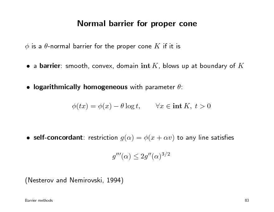
Normal barrier for proper cone
is a -normal barrier for the proper cone K if it is a barrier: smooth, convex, domain int K, blows up at boundary of K logarithmically homogeneous with parameter : (tx) = (x) log t, x int K, t > 0

self-concordant: restriction g() = (x + v) to any line satises g () 2g ()3/2 (Nesterov and Nemirovski, 1994)
Barrier methods 83

Examples
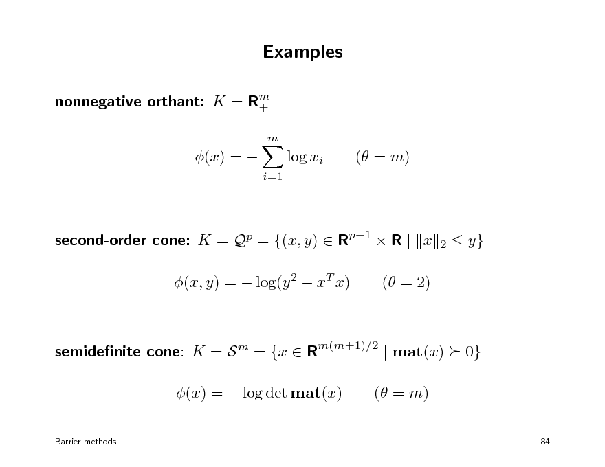
nonnegative orthant: K = Rm +
m

(x) =

log xi
i=1

( = m)

second-order cone: K = Qp = {(x, y) Rp1 R | x (x, y) = log(y 2 xT x) ( = 2)

2

y}

semidenite cone: K = S m = {x Rm(m+1)/2 | mat(x) (x) = log det mat(x)
Barrier methods

0}

( = m)
84

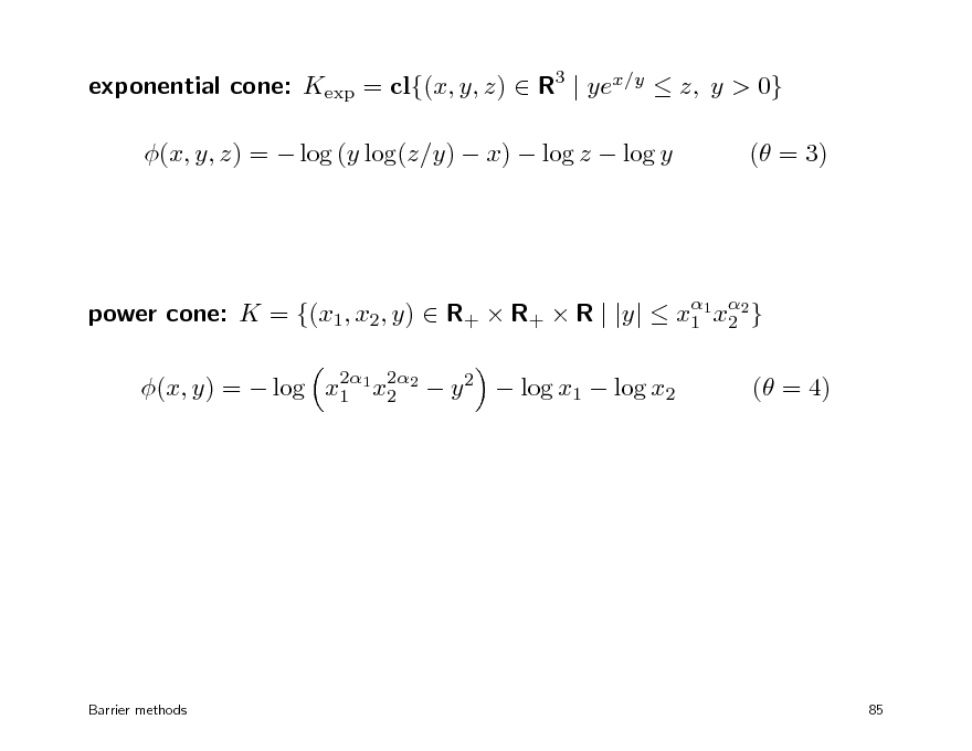
exponential cone: Kexp = cl{(x, y, z) R3 | yex/y z, y > 0} (x, y, z) = log (y log(z/y) x) log z log y ( = 3)

power cone: K = {(x1, x2, y) R+ R+ R | |y| x1 1 x2 } 2 2 2 (x, y) = log x1 1 x2 2 y 2 log x1 log x2

( = 4)

Barrier methods

85

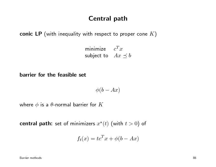
Central path
conic LP (with inequality with respect to proper cone K) minimize cT x subject to Ax barrier for the feasible set (b Ax) where is a -normal barrier for K central path: set of minimizers x(t) (with t > 0) of ft(x) = tcT x + (b Ax)
Barrier methods 86

b

Newton step
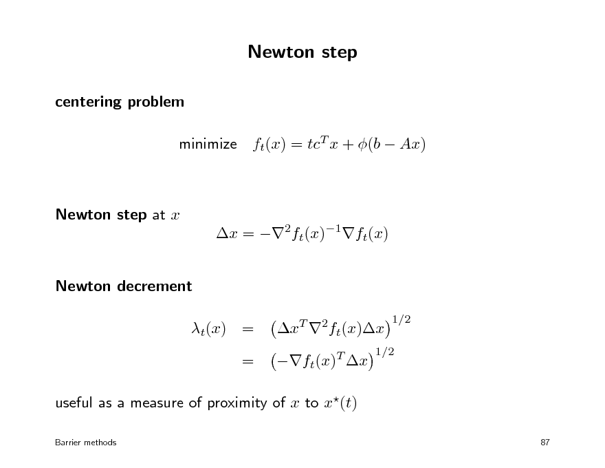
centering problem minimize ft(x) = tcT x + (b Ax)

Newton step at x x = 2ft(x)1ft(x) Newton decrement t(x) = = xT 2ft(x)x ft(x)T x
1/2

1/2

useful as a measure of proximity of x to x(t)
Barrier methods 87

Damped Newton method
minimize ft(x) = tcT x + (b Ax) algorithm (with parameters (0, 1/2), (0, 1/4]) select a starting point x dom ft repeat: 1. compute Newton step x and Newton decrement t(x) 2. if t(x)2 , return x 3. otherwise, set x := x + x with 1 = 1 + t(x) if t(x) , =1 if t(x) <

stopping criterion t(x)2 implies ft(x) inf ft(x) alternatively, can use backtracking line search
Barrier methods 88

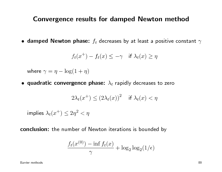
Convergence results for damped Newton method
damped Newton phase: ft decreases by at least a positive constant ft(x+) ft(x) where = log(1 + ) quadratic convergence phase: t rapidly decreases to zero 2t(x+) (2t(x)) implies t(x+) 2 2 < conclusion: the number of Newton iterations is bounded by ft(x(0)) inf ft(x) + log2 log2(1/)
Barrier methods 89

if t(x)

2

if t(x) <

Outline

barrier method for linear programming normal barriers barrier method for conic optimization

Central path and duality
x(t) = argmin tcT x + (b Ax) duality point on central path: x(t) denes a strictly dual feasible z (t) 1 z (t) = (s), t

s = b Ax(t)

duality gap: gap between x = x(t) and z = z (t) is c T x + bT z = s T z = , t
T

c T x p

t t(x) 1+ t

extension near central path (for t(x) < 1): c x p (results follow from properties of normal barriers)
Barrier methods

90

Short-step barrier method
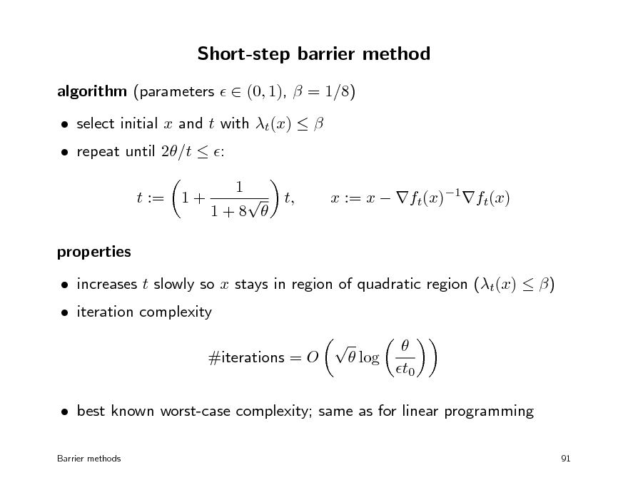
algorithm (parameters (0, 1), = 1/8) repeat until 2/t : t := properties increases t slowly so x stays in region of quadratic region (t(x) ) log t0 1+ select initial x and t with t(x) 1 t, 1+8

x := x ft(x)1ft(x)

iteration complexity

#iterations = O

best known worst-case complexity; same as for linear programming
Barrier methods 91

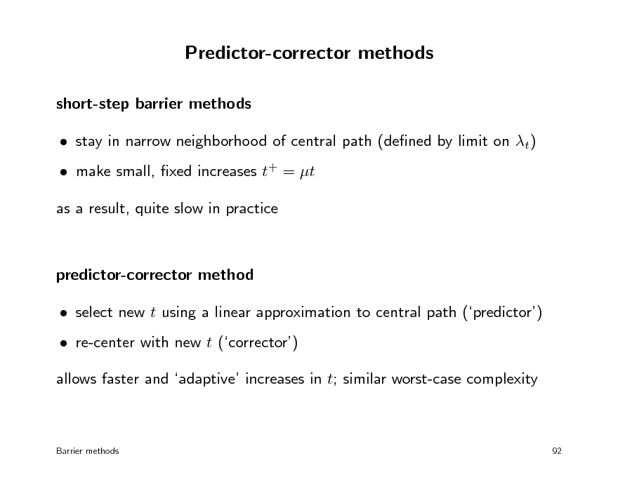
Predictor-corrector methods
short-step barrier methods stay in narrow neighborhood of central path (dened by limit on t) make small, xed increases t+ = t as a result, quite slow in practice

predictor-corrector method select new t using a linear approximation to central path (predictor) re-center with new t (corrector) allows faster and adaptive increases in t; similar worst-case complexity

Barrier methods

92

Convex optimization MLSS 2012

Primal-dual methods

primal-dual algorithms for linear programming symmetric cones primal-dual algorithms for conic optimization implementation

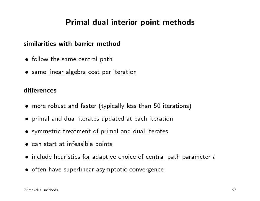
Primal-dual interior-point methods
similarities with barrier method follow the same central path same linear algebra cost per iteration dierences more robust and faster (typically less than 50 iterations) primal and dual iterates updated at each iteration symmetric treatment of primal and dual iterates can start at infeasible points include heuristics for adaptive choice of central path parameter t often have superlinear asymptotic convergence
Primal-dual methods 93

Primal-dual central path for linear programming
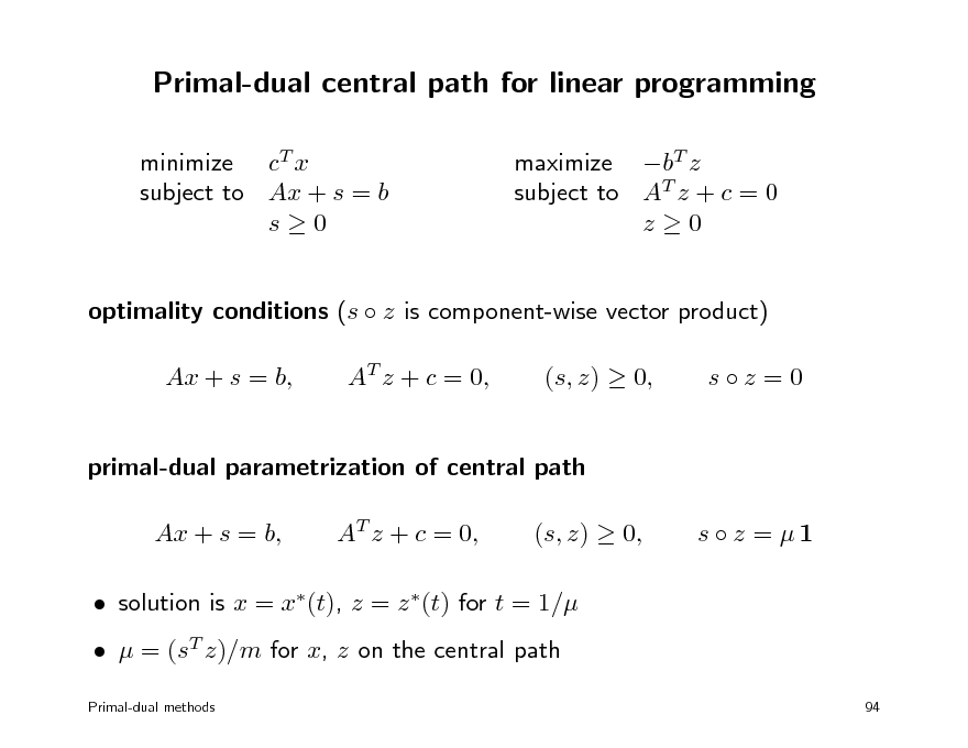
minimize cT x subject to Ax + s = b s0 maximize bT z subject to AT z + c = 0 z0

optimality conditions (s z is component-wise vector product) Ax + s = b, AT z + c = 0, (s, z) 0, sz =0

primal-dual parametrization of central path Ax + s = b, AT z + c = 0, (s, z) 0, s z = 1

solution is x = x(t), z = z (t) for t = 1/ = (sT z)/m for x, z on the central path
Primal-dual methods 94

Primal-dual search direction
current iterates x, s > 0, z > 0 updated as x := x + x, s := s + s, z := z + z

primal and dual steps x, s, z are dened by A( + x) + s + s = b, x AT ( + z) + c = 0 z

z s + s z = 1 s z where = (T z )/m and [0, 1] s last equation is linearization of ( + s) ( + z) = 1 s z dierent methods use dierent strategies for selecting (0, 1] selected so that s > 0, z > 0
Primal-dual methods 95

targets point on central path with = i.e., with gap (T z ) s

Linear algebra complexity
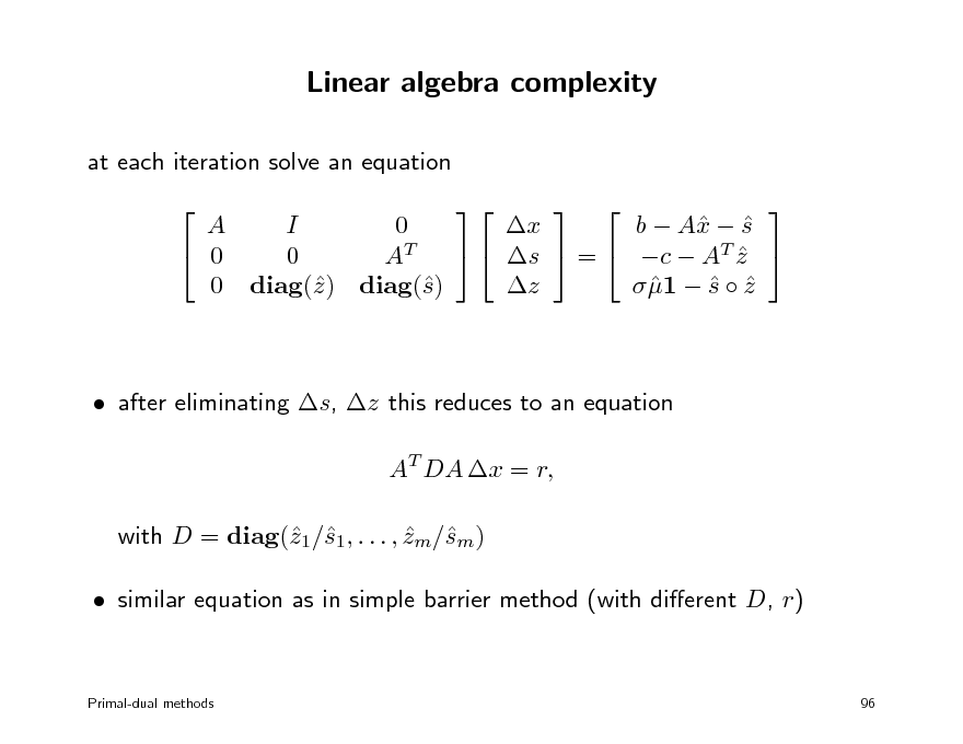
at each iteration solve an equation A I 0 b A s x x 0 s = c AT z 0 AT z 1 s z 0 diag() diag() z s after eliminating s, z this reduces to an equation AT DA x = r, with D = diag(1/1, . . . , zm/m) z s s similar equation as in simple barrier method (with dierent D, r)

Primal-dual methods

96

Outline

primal-dual algorithms for linear programming symmetric cones primal-dual algorithms for conic optimization implementation

Symmetric cones
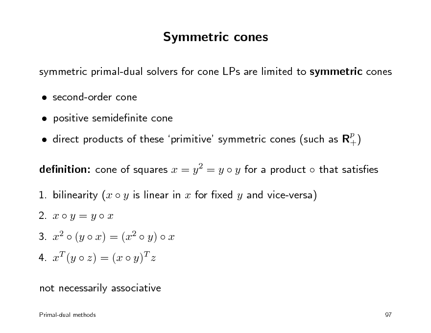
symmetric primal-dual solvers for cone LPs are limited to symmetric cones second-order cone positive semidenite cone direct products of these primitive symmetric cones (such as Rp ) + denition: cone of squares x = y 2 = y y for a product that satises 1. bilinearity (x y is linear in x for xed y and vice-versa) 2. x y = y x 3. x2 (y x) = (x2 y) x 4. xT (y z) = (x y)T z not necessarily associative
Primal-dual methods 97

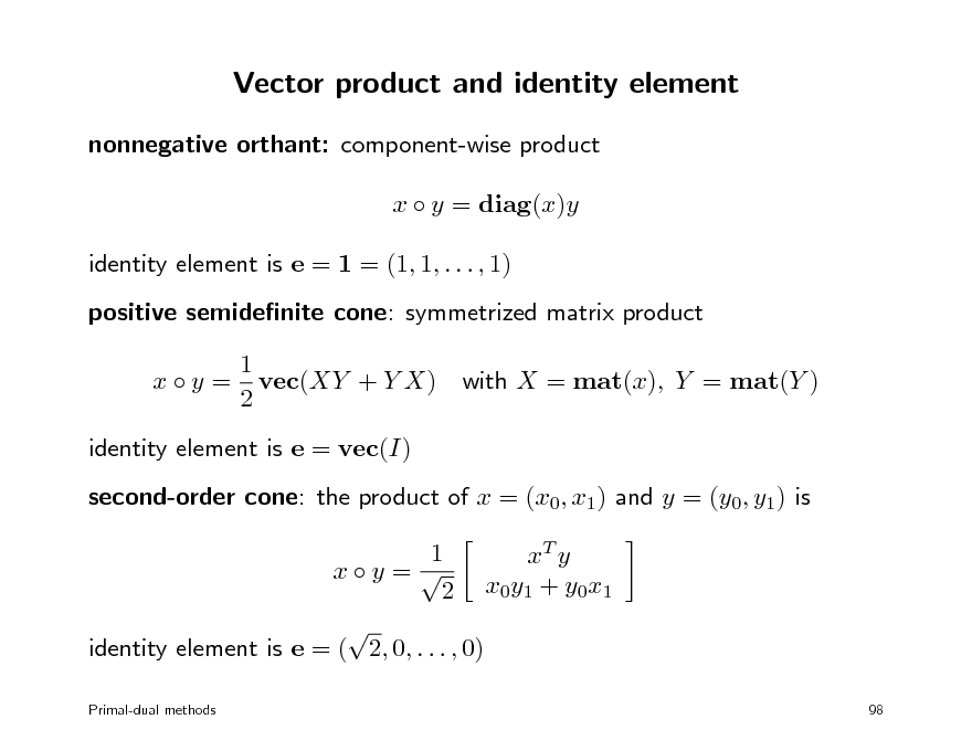
Vector product and identity element
nonnegative orthant: component-wise product x y = diag(x)y identity element is e = 1 = (1, 1, . . . , 1) positive semidenite cone: symmetrized matrix product 1 x y = vec(XY + Y X) 2 identity element is e = vec(I) second-order cone: the product of x = (x0, x1) and y = (y0, y1) is 1 xT y xy = 2 x0 y1 + y0 x1 identity element is e = ( 2, 0, . . . , 0)
Primal-dual methods 98

with X = mat(x), Y = mat(Y )

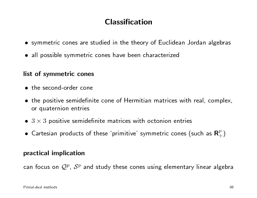
Classication
symmetric cones are studied in the theory of Euclidean Jordan algebras all possible symmetric cones have been characterized list of symmetric cones the second-order cone the positive semidenite cone of Hermitian matrices with real, complex, or quaternion entries 3 3 positive semidenite matrices with octonion entries Cartesian products of these primitive symmetric cones (such as Rp ) +

practical implication can focus on Qp, S p and study these cones using elementary linear algebra
Primal-dual methods 99

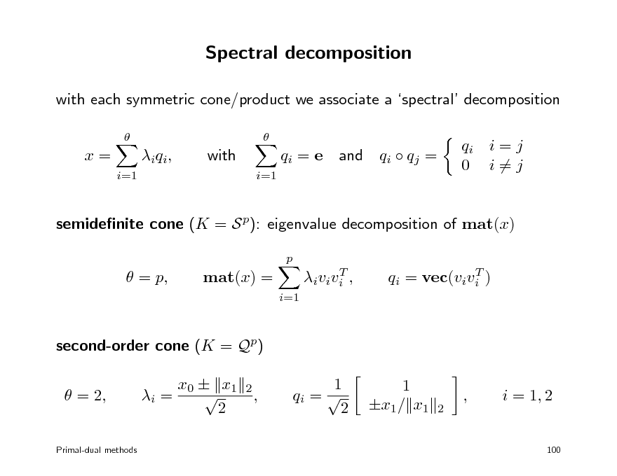
Spectral decomposition
with each symmetric cone/product we associate a spectral decomposition

x=
i=1

i q i ,

with
i=1

qi = e

and

qi qj =

qi i = j 0 i=j

semidenite cone (K = S p): eigenvalue decomposition of mat(x)
p

= p,

mat(x) =
i=1

T i v i v i ,

T qi = vec(vivi )

second-order cone (K = Qp) = 2, i = x0 x1 2
2

,

1 qi = 2

1 x1/ x1

2

,

i = 1, 2

Primal-dual methods

100

Applications
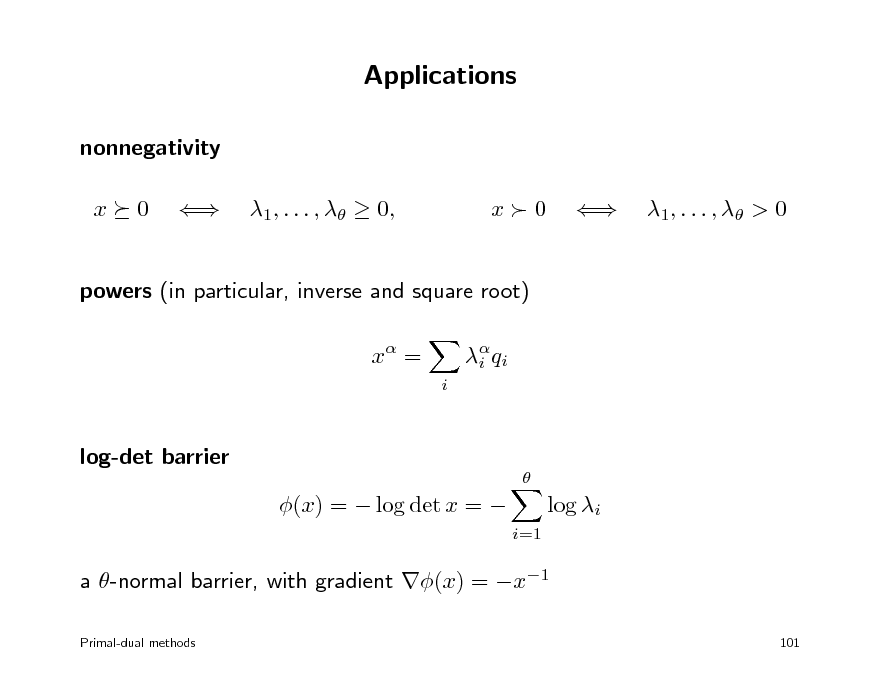
nonnegativity x 0 1, . . . , 0, x0 1 , . . . , > 0

powers (in particular, inverse and square root) x =
i i q i

log-det barrier

(x) = log det x =

log i
i=1

a -normal barrier, with gradient (x) = x1
Primal-dual methods 101

Outline

primal-dual algorithms for linear programming symmetric cones primal-dual algorithms for conic optimization implementation

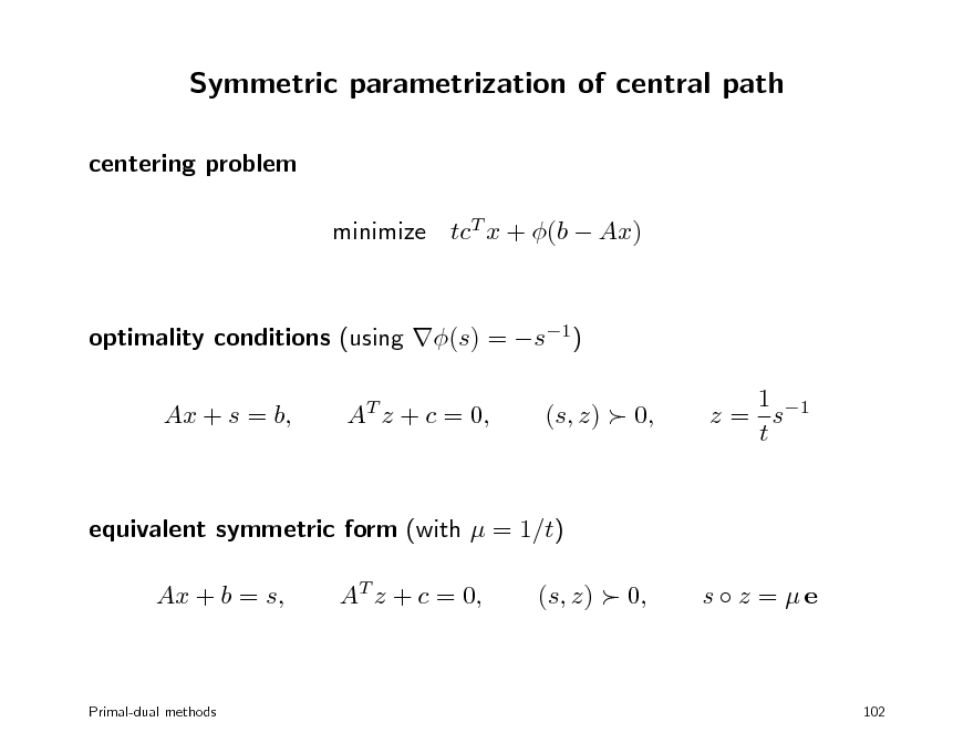
Symmetric parametrization of central path
centering problem minimize tcT x + (b Ax) optimality conditions (using (s) = s1) Ax + s = b, AT z + c = 0, (s, z) 0, 1 z = s1 t

equivalent symmetric form (with = 1/t) Ax + b = s, AT z + c = 0, (s, z) 0, s z = e

Primal-dual methods

102

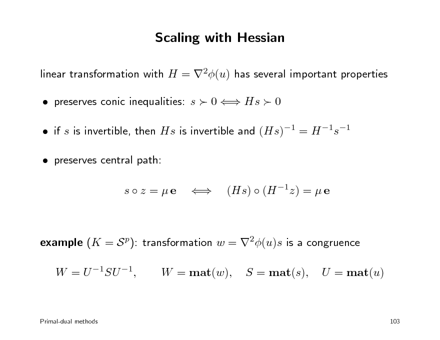
Scaling with Hessian
linear transformation with H = 2(u) has several important properties preserves conic inequalities: s 0 Hs 0 if s is invertible, then Hs is invertible and (Hs)1 = H 1s1 preserves central path: s z = e (Hs) (H 1z) = e

example (K = S p): transformation w = 2(u)s is a congruence W = U 1SU 1, W = mat(w), S = mat(s), U = mat(u)

Primal-dual methods

103

Primal-dual search direction
steps x, s, z at current iterates x, s, z are dened by A( + x) + s + s = b, x AT ( + z) + c = 0 z

(H s) (H 1z) + (H 1z ) (Hs) = e (H s) (H 1z ) where = (T z )/, [0, 1], and H = 2(u) s last equation is linearization of (H( + s)) H 1( + z) = e s z dierent algorithms use dierent choices of , H Nesterov-Todd scaling: choose H = 2(u) such that H s = H 1z
Primal-dual methods 104

Outline

primal-dual algorithms for linear programming symmetric cones primal-dual algorithms for conic optimization implementation

Software implementations
general-purpose software for nonlinear convex optimization several high-quality packages (MOSEK, Sedumi, SDPT3, SDPA, . . . ) exploit sparsity to achieve scalability

customized implementations can exploit non-sparse types of problem structure often orders of magnitude faster than general-purpose solvers

Primal-dual methods

105

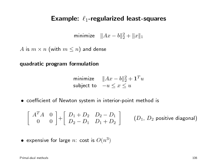
Example: 1-regularized least-squares
minimize Ax b
2 2

+ x

1

A is m n (with m n) and dense quadratic program formulation minimize Ax b 2 + 1T u 2 subject to u x u coecient of Newton system in interior-point method is AT A 0 0 0 + D1 + D2 D2 D1 D2 D1 D1 + D2 (D1, D2 positive diagonal)

expensive for large n: cost is O(n3)
Primal-dual methods 106

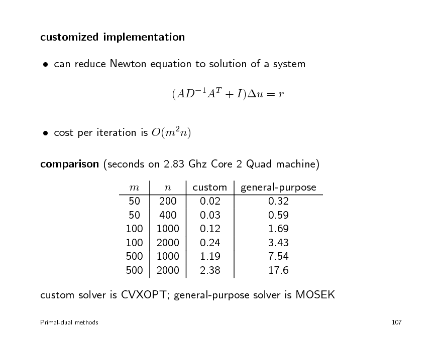
customized implementation can reduce Newton equation to solution of a system (AD1AT + I)u = r cost per iteration is O(m2n) comparison (seconds on 2.83 Ghz Core 2 Quad machine) m 50 50 100 100 500 500 n 200 400 1000 2000 1000 2000 custom 0.02 0.03 0.12 0.24 1.19 2.38 general-purpose 0.32 0.59 1.69 3.43 7.54 17.6

custom solver is CVXOPT; general-purpose solver is MOSEK
Primal-dual methods 107

Overview

1. Basic theory and convex modeling convex sets and functions common problem classes and applications 2. Interior-point methods for conic optimization conic optimization barrier methods symmetric primal-dual methods 3. First-order methods (proximal) gradient algorithms dual techniques and multiplier methods

Convex optimization MLSS 2012

Gradient methods

gradient and subgradient method proximal gradient method fast proximal gradient methods

108

Classical gradient method
to minimize a convex dierentiable function f : choose x(0) and repeat x(k) = x(k1) tk f (x(k1)), step size tk is constant or from line search advantages every iteration is inexpensive does not require second derivatives disadvantages often very slow; very sensitive to scaling does not handle nondierentiable functions
Gradient methods 109

k = 1, 2, . . .

Quadratic example
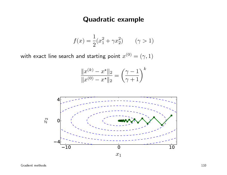
1 2 f (x) = (x1 + x2) 2 2 ( > 1)

with exact line search and starting point x(0) = (, 1) x(k) x x(0) x
4 0 4

2 2

=

1 +1

k

x2

10

0 x1

10
110

Gradient methods

Nondierentiable example
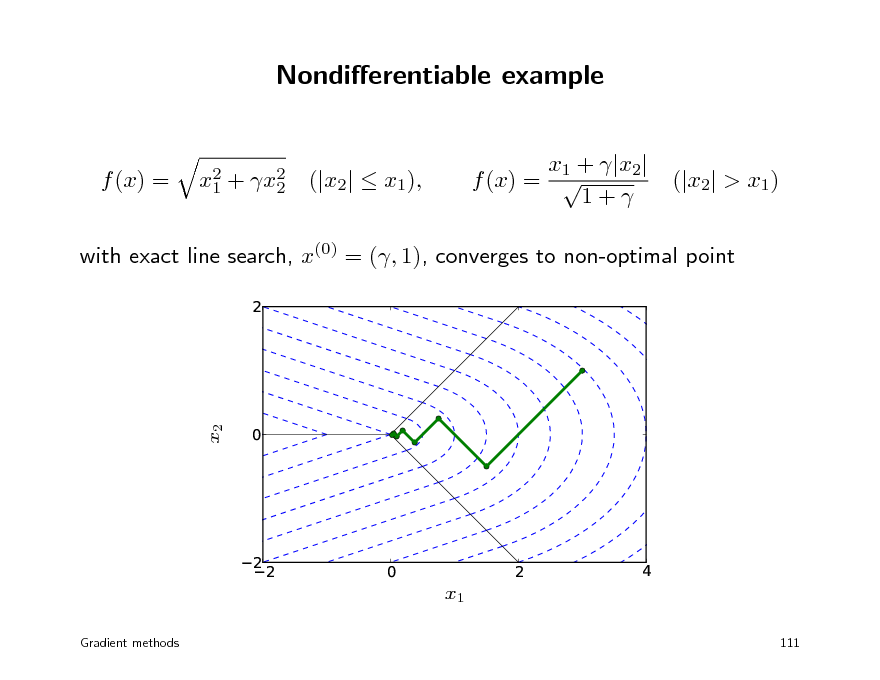
x1 + |x2| f (x) = 1+

f (x) =

x2 + x2 1 2

(|x2| x1),

(|x2| > x1)

with exact line search, x(0) = (, 1), converges to non-optimal point
2

0

x2

22

0

2

4

x1
Gradient methods 111

First-order methods
address one or both disadvantages of the gradient method methods for nondierentiable or constrained problems smoothing methods subgradient method proximal gradient method methods with improved convergence variable metric methods conjugate gradient method accelerated proximal gradient method we will discuss subgradient and proximal gradient methods
Gradient methods 112

Subgradient
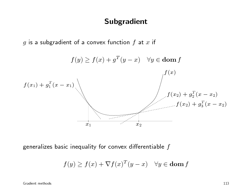
g is a subgradient of a convex function f at x if f (y) f (x) + g T (y x)
T f (x1) + g1 (x x1) T f (x2) + g2 (x x2) T f (x2) + g3 (x x2)

y dom f
f (x)

x1

x2

generalizes basic inequality for convex dierentiable f f (y) f (x) + f (x)T (y x)
Gradient methods

y dom f
113

Subdierential
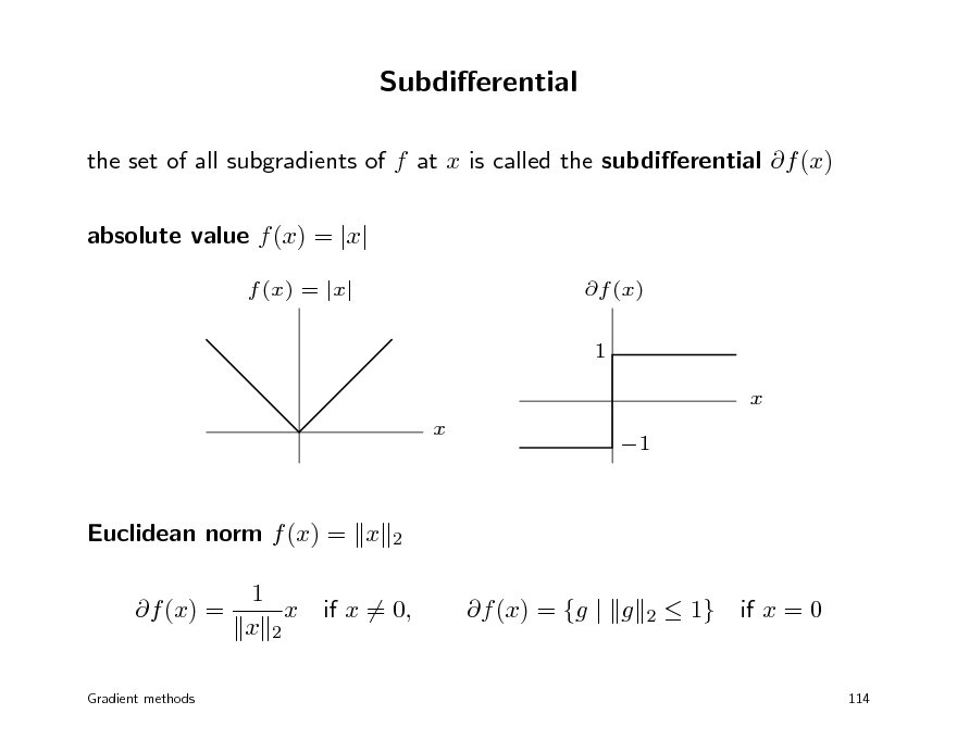
the set of all subgradients of f at x is called the subdierential f (x) absolute value f (x) = |x|
f (x) = |x| f (x) 1 x x 1

Euclidean norm f (x) = x f (x) = 1 x x 2

2

if x = 0,

f (x) = {g | g

2

1}

if x = 0

Gradient methods

114

Subgradient calculus
weak calculus rules for nding one subgradient sucient for most algorithms for nondierentiable convex optimization if one can evaluate f (x), one can usually compute a subgradient much easier than nding the entire subdierential

subdierentiability convex f is subdierentiable on dom f except possibly at the boundary example of a non-subdierentiable function: f (x) = x at x = 0

Gradient methods

115

Examples of calculus rules
nonnegative combination: f = 1f1 + 2f2 with 1, 2 0 g = 1 g1 + 2 g2 , g1 f1(x), g2 f2(x)

composition with ane transformation: f (x) = h(Ax + b) g = AT g , g h(Ax + b)

pointwise maximum f (x) = max{f1(x), . . . , fm(x)} g fi(x) where fi(x) = max fk (x)
k

conjugate f (x) = supy (xT y f (y)): take any maximizing y
Gradient methods 116

Subgradient method
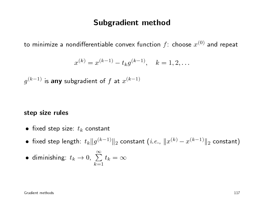
to minimize a nondierentiable convex function f : choose x(0) and repeat x(k) = x(k1) tk g (k1), g (k1) is any subgradient of f at x(k1) k = 1, 2, . . .

step size rules xed step size: tk constant xed step length: tk g (k1)
2

constant (i.e., x(k) x(k1)

2

constant)

diminishing: tk 0,

k=1

tk =

Gradient methods

117

Some convergence results
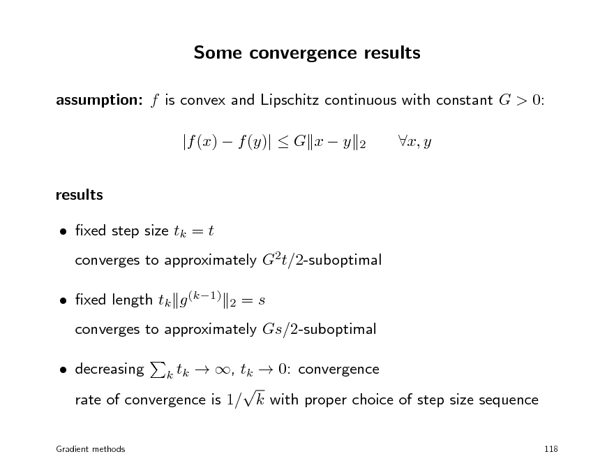
assumption: f is convex and Lipschitz continuous with constant G > 0: |f (x) f (y)| G x y results xed step size tk = t
2

x, y

converges to approximately G2t/2-suboptimal
2

xed length tk g (k1)

=s

converges to approximately Gs/2-suboptimal decreasing , tk 0: convergence rate of convergence is 1/ k with proper choice of step size sequence
k tk
118

Gradient methods

Example: 1-norm minimization
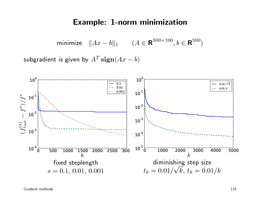
minimize Ax b
1

(A R500100, b R500)

subgradient is given by AT sign(Ax b)
10
0
0.1 0.01 0.001

10

0

0.01/ 0.01/k

k

(fbest f )/f

10

-1

10

-1

10 10
-2

-2

(k)

10 10
-3

-3

10

-4

10

-4

0

500

1000

1500

k

2000

2500

3000

10

-5

0

1000

2000

k

3000

4000

5000

xed steplength s = 0.1, 0.01, 0.001
Gradient methods

diminishing step size tk = 0.01/ k, tk = 0.01/k
119

Outline

gradient and subgradient method proximal gradient method fast proximal gradient methods

Proximal operator
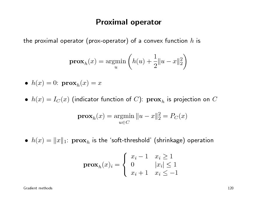
the proximal operator (prox-operator) of a convex function h is proxh(x) = argmin h(u) +
u

1 ux 2

2 2

h(x) = 0: proxh(x) = x h(x) = IC (x) (indicator function of C): proxh is projection on C proxh(x) = argmin u x
uC 2 2

= PC (x)

h(x) = x 1: proxh is the soft-threshold (shrinkage) operation xi 1 xi 1 0 |xi| 1 proxh(x)i = xi + 1 xi 1

Gradient methods

120

Proximal gradient method
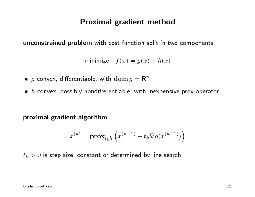
unconstrained problem with cost function split in two components minimize f (x) = g(x) + h(x) g convex, dierentiable, with dom g = Rn h convex, possibly nondierentiable, with inexpensive prox-operator proximal gradient algorithm x(k) = proxtk h x(k1) tk g(x(k1)) tk > 0 is step size, constant or determined by line search

Gradient methods

121

Examples
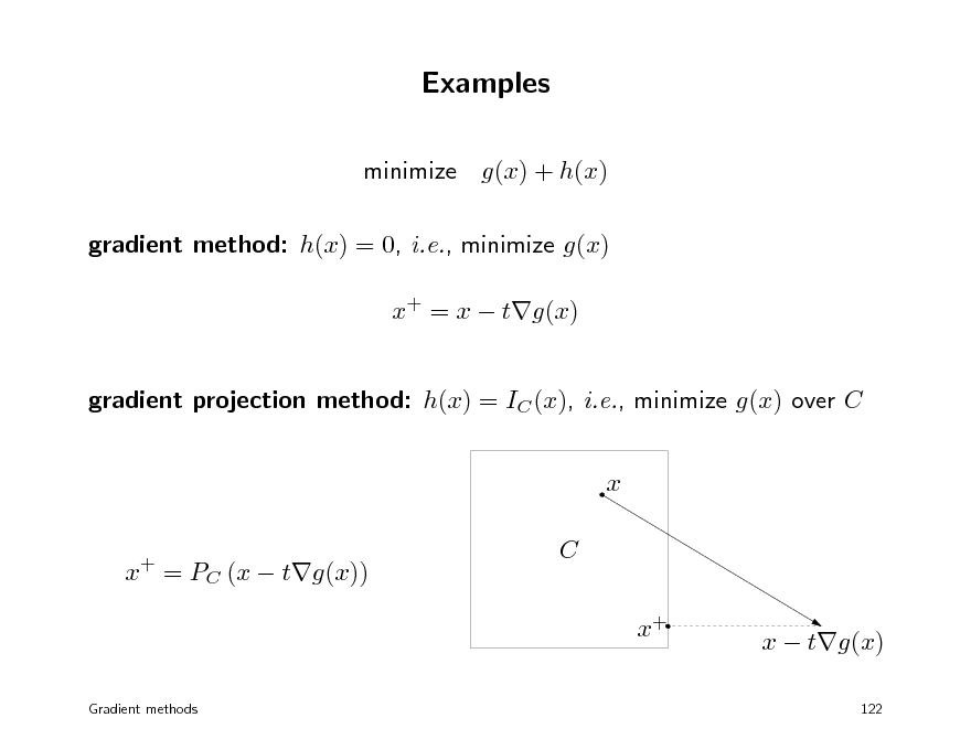
minimize g(x) + h(x) gradient method: h(x) = 0, i.e., minimize g(x) x+ = x tg(x) gradient projection method: h(x) = IC (x), i.e., minimize g(x) over C x x = PC (x tg(x))
+

C x+

x tg(x)
122

Gradient methods

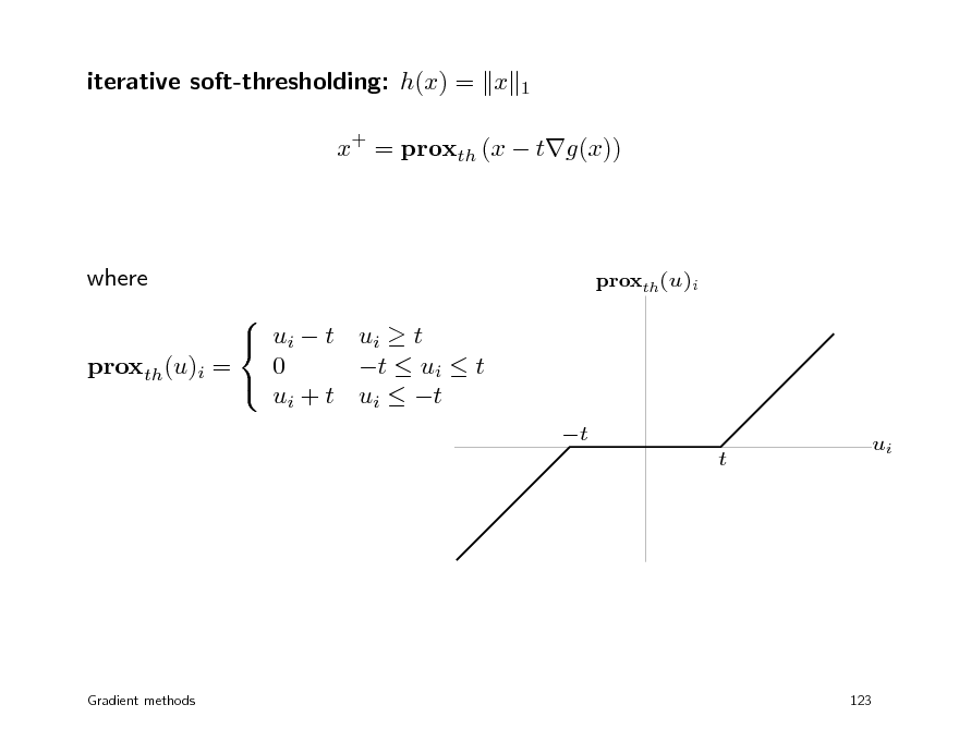
iterative soft-thresholding: h(x) = x

1

x+ = proxth (x tg(x))

where ui t ui t 0 t ui t proxth(u)i = ui + t ui t

proxth(u)i

t t

ui

Gradient methods

123

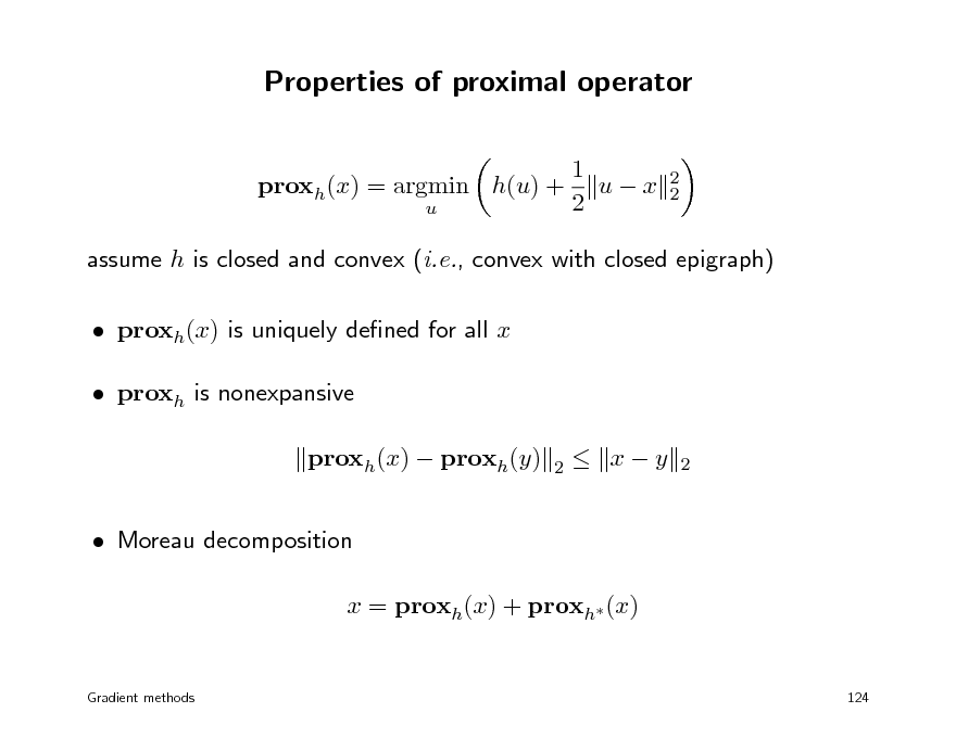
Properties of proximal operator
1 proxh(x) = argmin h(u) + u x 2 u
2 2

assume h is closed and convex (i.e., convex with closed epigraph) proxh(x) is uniquely dened for all x proxh is nonexpansive proxh(x) proxh(y) Moreau decomposition x = proxh(x) + proxh (x)
2

xy

2

Gradient methods

124

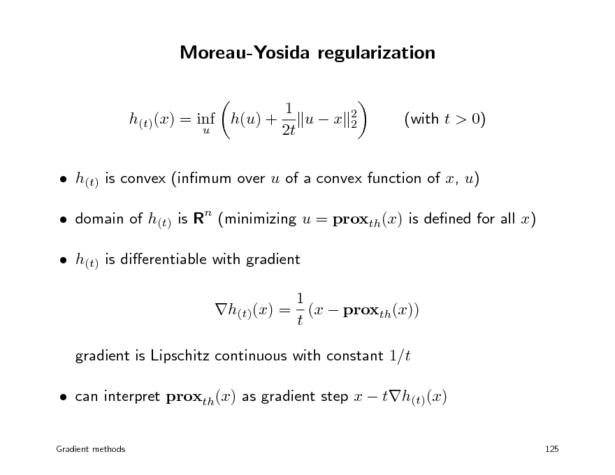
Moreau-Yosida regularization
1 ux 2t
2 2

h(t)(x) = inf h(u) +
u

(with t > 0)

h(t) is convex (inmum over u of a convex function of x, u) domain of h(t) is Rn (minimizing u = proxth(x) is dened for all x) h(t) is dierentiable with gradient 1 h(t)(x) = (x proxth(x)) t gradient is Lipschitz continuous with constant 1/t can interpret proxth(x) as gradient step x th(t)(x)
Gradient methods 125

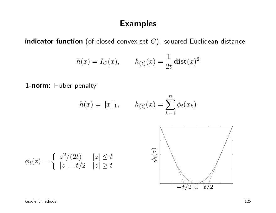
Examples
indicator function (of closed convex set C): squared Euclidean distance h(x) = IC (x), 1-norm: Huber penalty
n

h(t)(x) =

1 dist(x)2 2t

h(x) = x 1,

h(t)(x) =
k=1

t(xk )

t(z) =

z 2/(2t) |z| t |z| t/2 |z| t

t(z)

t/2 z t/2
Gradient methods 126

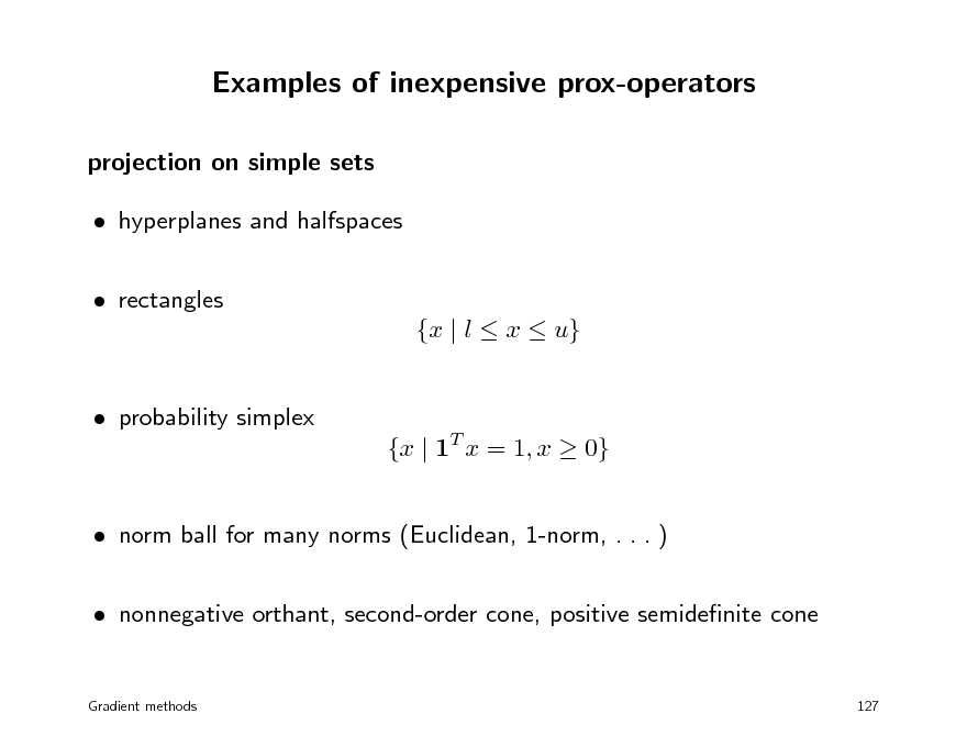
Examples of inexpensive prox-operators
projection on simple sets hyperplanes and halfspaces rectangles

{x | l x u}

probability simplex

{x | 1T x = 1, x 0}

norm ball for many norms (Euclidean, 1-norm, . . . ) nonnegative orthant, second-order cone, positive semidenite cone
Gradient methods 127

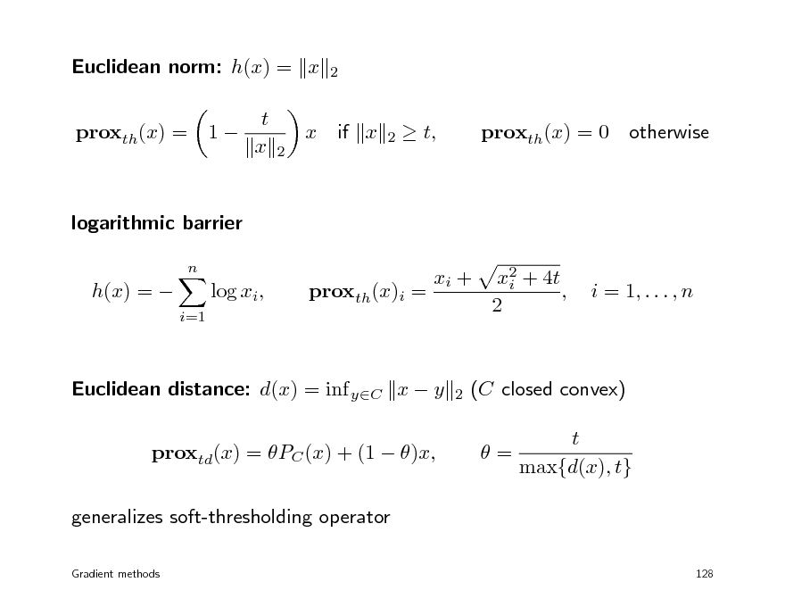
Euclidean norm: h(x) = x proxth(x) = 1 t x x
2

2

if x

2

t,

proxth(x) = 0

otherwise

logarithmic barrier
n

h(x) =

log xi,
i=1

proxth(x)i =

xi +

x2 + 4t i , 2

i = 1, . . . , n

Euclidean distance: d(x) = inf yC x y proxtd(x) = PC (x) + (1 )x, generalizes soft-thresholding operator
Gradient methods

2

(C closed convex) = t max{d(x), t}

128

Prox-operator of conjugate
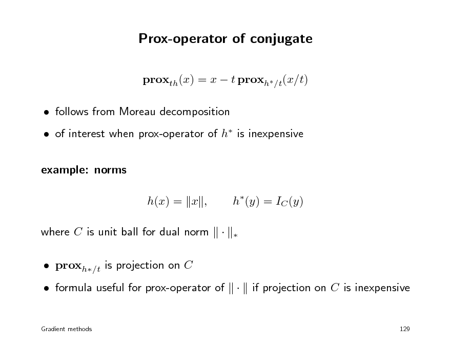
proxth(x) = x t proxh/t(x/t) follows from Moreau decomposition of interest when prox-operator of h is inexpensive example: norms h(x) = x , where C is unit ball for dual norm proxh/t is projection on C formula useful for prox-operator of
Gradient methods

h(y) = IC (y)

if projection on C is inexpensive

129

Support function
many convex functions can be expressed as support functions h(x) = SC (x) = sup xT y
yC

with C closed, convex conjugate is indicator function of C: h(y) = IC (y) hence, can compute proxth via projection on C example: h(x) is sum of largest r components of x h(x) = x[1] + + x[r] = SC (x), C = {y | 0 y 1, 1T y = r}

Gradient methods

130

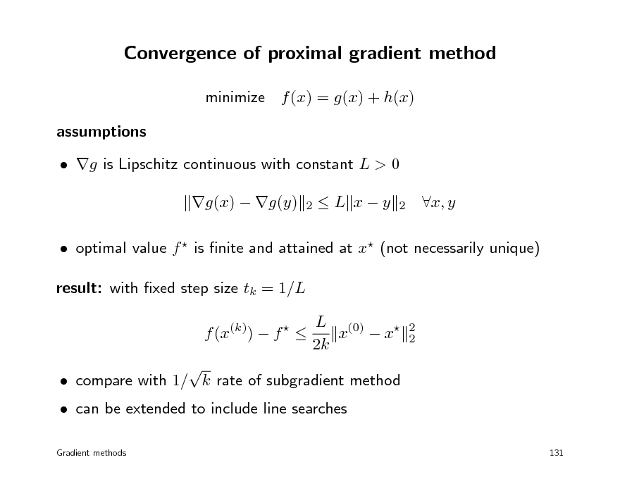
Convergence of proximal gradient method
minimize f (x) = g(x) + h(x) assumptions g is Lipschitz continuous with constant L > 0 g(x) g(y)
2

L xy

2

x, y

optimal value f is nite and attained at x (not necessarily unique) result: with xed step size tk = 1/L f (x(k)) f L (0) x x 2k
2 2

can be extended to include line searches
Gradient methods

compare with 1/ k rate of subgradient method

131

Outline

gradient and subgradient method proximal gradient method fast proximal gradient methods

Fast (proximal) gradient methods

Nesterov (1983, 1988, 2005): three gradient projection methods with 1/k 2 convergence rate Beck & Teboulle (2008): FISTA, a proximal gradient version of Nesterovs 1983 method Nesterov (2004 book), Tseng (2008): overview and unied analysis of fast gradient methods several recent variations and extensions this lecture: FISTA (Fast Iterative Shrinkage-Thresholding Algorithm)

Gradient methods

132

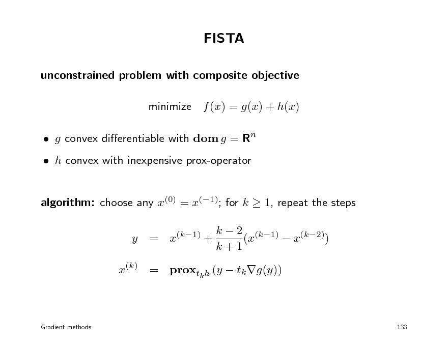
FISTA
unconstrained problem with composite objective minimize f (x) = g(x) + h(x) g convex dierentiable with dom g = Rn h convex with inexpensive prox-operator algorithm: choose any x(0) = x(1); for k 1, repeat the steps y = x(k1) + k 2 (k1) (x x(k2)) k+1

x(k) = proxtk h (y tk g(y))

Gradient methods

133

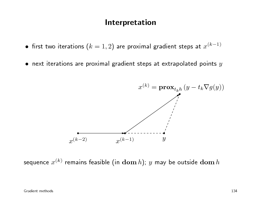
Interpretation
rst two iterations (k = 1, 2) are proximal gradient steps at x(k1) next iterations are proximal gradient steps at extrapolated points y x(k) = proxtk h (y tk g(y))

x(k2)

x(k1)

y

sequence x(k) remains feasible (in dom h); y may be outside dom h

Gradient methods

134

Convergence of FISTA
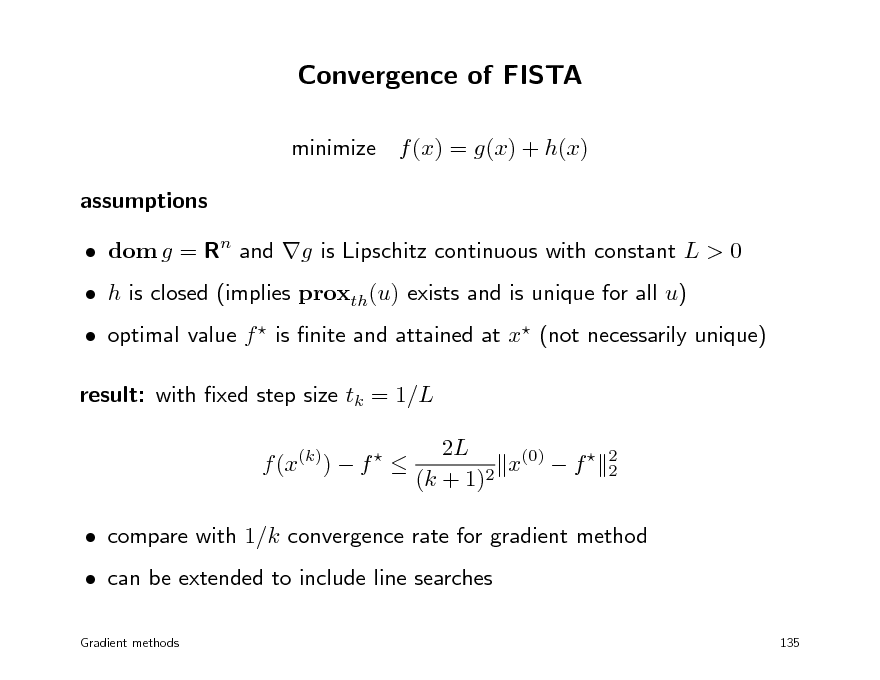
minimize f (x) = g(x) + h(x) assumptions dom g = Rn and g is Lipschitz continuous with constant L > 0 optimal value f is nite and attained at x (not necessarily unique) result: with xed step size tk = 1/L f (x(k)) f 2L x(0) f (k + 1)2
2 2

h is closed (implies proxth(u) exists and is unique for all u)

compare with 1/k convergence rate for gradient method can be extended to include line searches
Gradient methods 135

Example
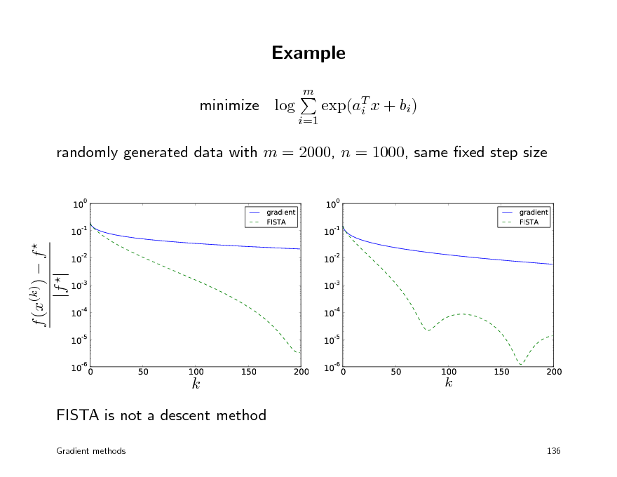
m

minimize log
i=1

exp(aT x + bi) i

randomly generated data with m = 2000, n = 1000, same xed step size
100 10-1 100 10-1 10-2 10-3 10-4 10-5 50 100 150 200 10-6 0 50 100 150 200

gradient FISTA

gradient FISTA

f (x(k)) f |f |

10-2 10-3 10-4 10-5 10-6 0

k

k

FISTA is not a descent method
Gradient methods 136

Convex optimization MLSS 2012

Dual methods

Lagrange duality dual decomposition dual proximal gradient method multiplier methods

Dual function
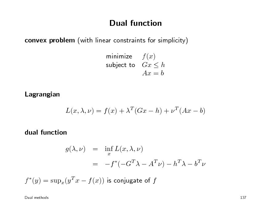
convex problem (with linear constraints for simplicity) minimize f (x) subject to Gx h Ax = b Lagrangian L(x, , ) = f (x) + T (Gx h) + T (Ax b) dual function g(, ) = inf L(x, , )
x

= f (GT AT ) hT bT f (y) = supx(y T x f (x)) is conjugate of f
Dual methods 137

Dual problem
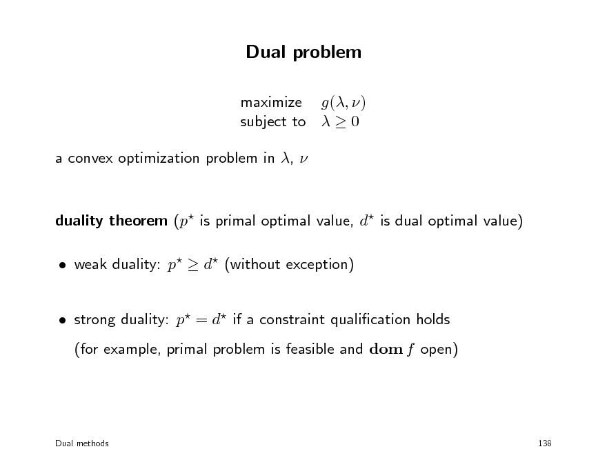
maximize g(, ) subject to 0 a convex optimization problem in ,

duality theorem (p is primal optimal value, d is dual optimal value) weak duality: p d (without exception) strong duality: p = d if a constraint qualication holds (for example, primal problem is feasible and dom f open)

Dual methods

138

Norm approximation
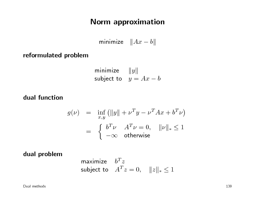
minimize reformulated problem minimize y subject to y = Ax b dual function g() = inf = dual problem
x,y

Ax b

y + T y T Ax + bT bT AT = 0, otherwise

1

maximize bT z subject to AT z = 0,

z

1
139

Dual methods

Karush-Kuhn-Tucker optimality conditions
if strong duality holds, then x, , are optimal if and only if 1. x is primal feasible x dom f, 2. 0 3. complementary slackness holds T (h Gx) = 0 4. x minimizes L(x, , ) = f (x) + T (Gx h) + T (Ax b) for dierentiable f , condition 4 can be expressed as f (x) + GT + AT = 0
Dual methods 140

Gx h,

Ax = b

Outline

Lagrange dual dual decomposition dual proximal gradient method multiplier methods

Dual methods
primal problem minimize f (x) subject to Gx h Ax = b dual problem maximize hT bT f (GT AT ) subject to 0 possible advantages of solving the dual when using rst-order methods dual problem is unconstrained or has simple constraints dual is dierentiable dual (almost) decomposes into smaller problems
Dual methods 141

(Sub-)gradients of conjugate function
f (y) = sup y T x f (x)
x

subgradient: x is a subgradient at y if it maximizes y T x f (x) if maximizing x is unique, then f is dierentiable at y this is the case, for example, if f is strictly convex

strongly convex function: f is strongly convex with modulus > 0 if T f (x) x x 2 is convex

implies that f (x) is Lipschitz continuous with parameter 1/

Dual methods

142

Dual gradient method
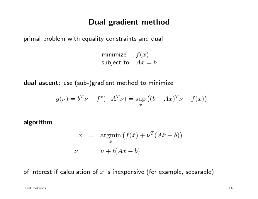
primal problem with equality constraints and dual minimize f (x) subject to Ax = b dual ascent: use (sub-)gradient method to minimize g() = bT + f (AT ) = sup (b Ax)T f (x)
x

algorithm x x x = argmin f () + T (A b)
x

+ = + t(Ax b) of interest if calculation of x is inexpensive (for example, separable)
Dual methods 143

Dual decomposition
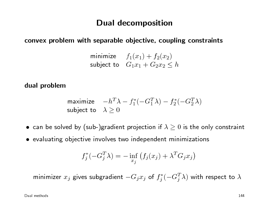
convex problem with separable objective, coupling constraints minimize f1(x1) + f2(x2) subject to G1x1 + G2x2 h dual problem
maximize hT f1 (GT ) f2 (GT ) 1 2 subject to 0

can be solved by (sub-)gradient projection if 0 is the only constraint evaluating objective involves two independent minimizations
fj (GT ) = inf fj (xj ) + T Gj xj j xj T minimizer xj gives subgradient Gj xj of fj (Gj ) with respect to
Dual methods 144

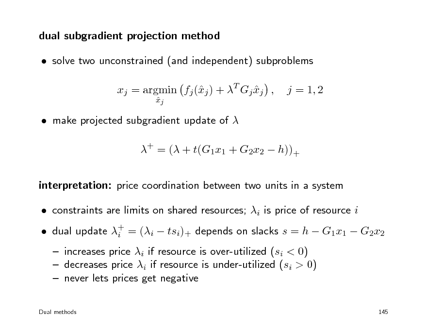
dual subgradient projection method solve two unconstrained (and independent) subproblems xj = argmin fj (j ) + T Gj xj , x
xj

j = 1, 2

make projected subgradient update of + = ( + t(G1x1 + G2x2 h))+ interpretation: price coordination between two units in a system constraints are limits on shared resources; i is price of resource i increases price i if resource is over-utilized (si < 0) decreases price i if resource is under-utilized (si > 0) never lets prices get negative
Dual methods 145

dual update + = (i tsi)+ depends on slacks s = h G1x1 G2x2 i

Outline

Lagrange dual dual decomposition dual proximal gradient method multiplier methods

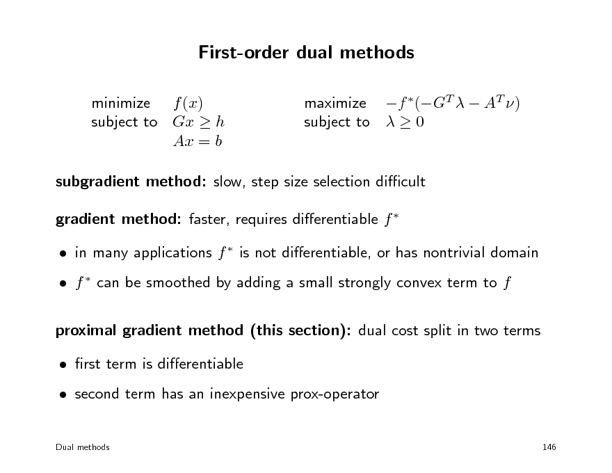
First-order dual methods
minimize f (x) subject to Gx h Ax = b maximize f (GT AT ) subject to 0

subgradient method: slow, step size selection dicult gradient method: faster, requires dierentiable f in many applications f is not dierentiable, or has nontrivial domain f can be smoothed by adding a small strongly convex term to f proximal gradient method (this section): dual cost split in two terms rst term is dierentiable second term has an inexpensive prox-operator
Dual methods 146

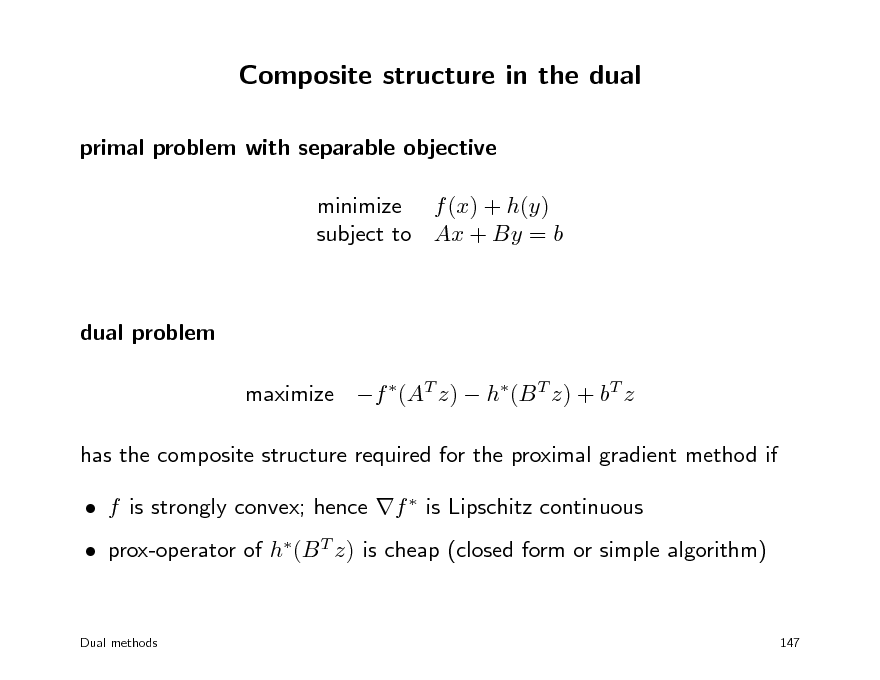
Composite structure in the dual
primal problem with separable objective minimize f (x) + h(y) subject to Ax + By = b

dual problem maximize f (AT z) h(B T z) + bT z has the composite structure required for the proximal gradient method if f is strongly convex; hence f is Lipschitz continuous prox-operator of h(B T z) is cheap (closed form or simple algorithm)

Dual methods

147

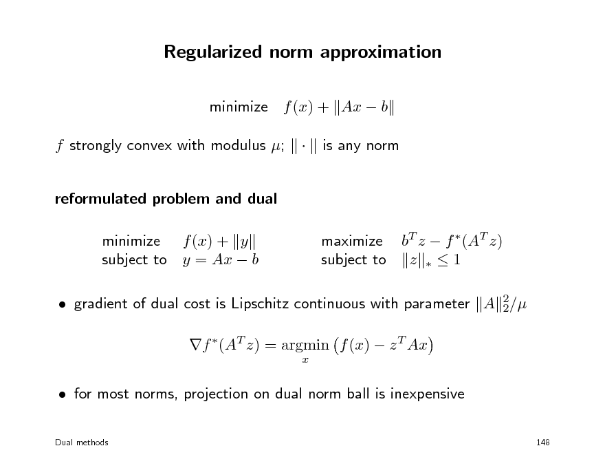
Regularized norm approximation
minimize f (x) + Ax b f strongly convex with modulus ; reformulated problem and dual minimize f (x) + y subject to y = Ax b maximize bT z f (AT z) subject to z 1 is any norm

gradient of dual cost is Lipschitz continuous with parameter A 2/ 2 f (AT z) = argmin f (x) z T Ax
x

for most norms, projection on dual norm ball is inexpensive
Dual methods 148

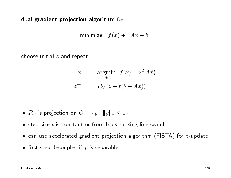
dual gradient projection algorithm for minimize f (x) + Ax b choose initial z and repeat x x x = argmin f () z T A
x

z + = PC (z + t(b Ax))

PC is projection on C = {y | y

1}

step size t is constant or from backtracking line search can use accelerated gradient projection algorithm (FISTA) for z-update rst step decouples if f is separable
Dual methods 149

Outline

Lagrange dual dual decomposition dual proximal gradient method multiplier methods

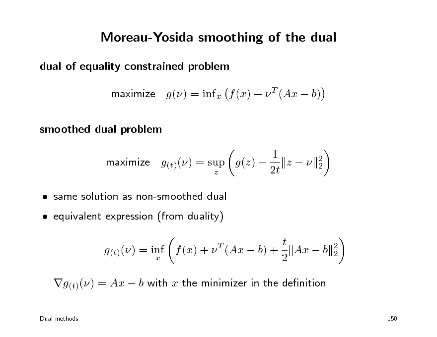
Moreau-Yosida smoothing of the dual
dual of equality constrained problem maximize g() = inf x f (x) + T (Ax b) smoothed dual problem 1 maximize g(t)() = sup g(z) z 2t z same solution as non-smoothed dual equivalent expression (from duality) g(t)() = inf f (x) + T (Ax b) +
x 2 2

t Ax b 2

2 2

g(t)() = Ax b with x the minimizer in the denition
Dual methods 150

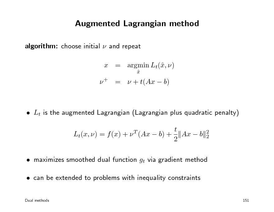
Augmented Lagrangian method
algorithm: choose initial and repeat x = argmin Lt(, ) x
x

+ = + t(Ax b)

Lt is the augmented Lagrangian (Lagrangian plus quadratic penalty) t Lt(x, ) = f (x) + (Ax b) + Ax b 2
T 2 2

maximizes smoothed dual function gt via gradient method can be extended to problems with inequality constraints
Dual methods 151

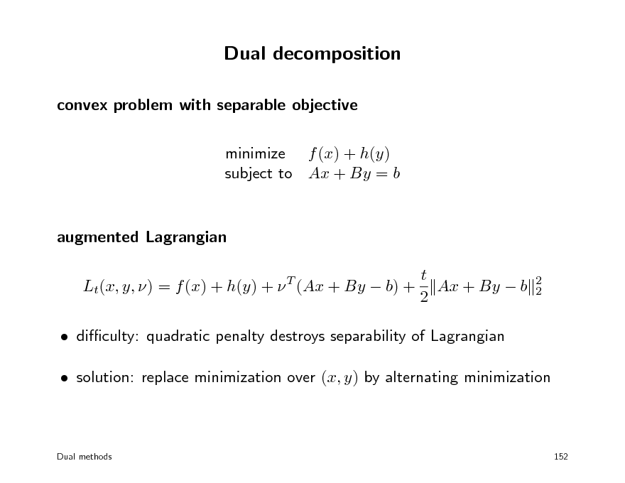
Dual decomposition
convex problem with separable objective minimize f (x) + h(y) subject to Ax + By = b

augmented Lagrangian t Lt(x, y, ) = f (x) + h(y) + (Ax + By b) + Ax + By b 2
T 2 2

diculty: quadratic penalty destroys separability of Lagrangian solution: replace minimization over (x, y) by alternating minimization

Dual methods

152

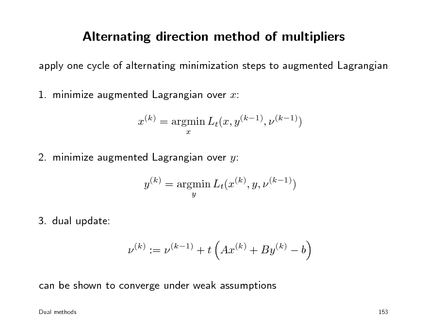
Alternating direction method of multipliers
apply one cycle of alternating minimization steps to augmented Lagrangian 1. minimize augmented Lagrangian over x: x(k) = argmin Lt(x, y (k1), (k1))
x

2. minimize augmented Lagrangian over y: y (k) = argmin Lt(x(k), y, (k1))
y

3. dual update: (k) := (k1) + t Ax(k) + By (k) b can be shown to converge under weak assumptions
Dual methods 153

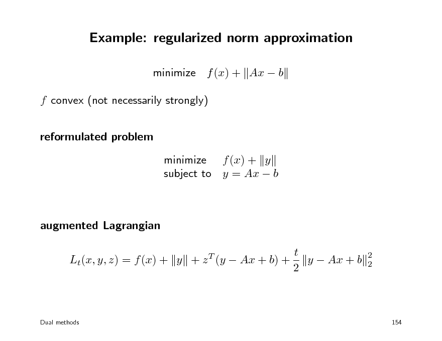
Example: regularized norm approximation
minimize f (x) + Ax b f convex (not necessarily strongly) reformulated problem minimize f (x) + y subject to y = Ax b

augmented Lagrangian t y Ax + b Lt(x, y, z) = f (x) + y + z (y Ax + b) + 2
T 2 2

Dual methods

154

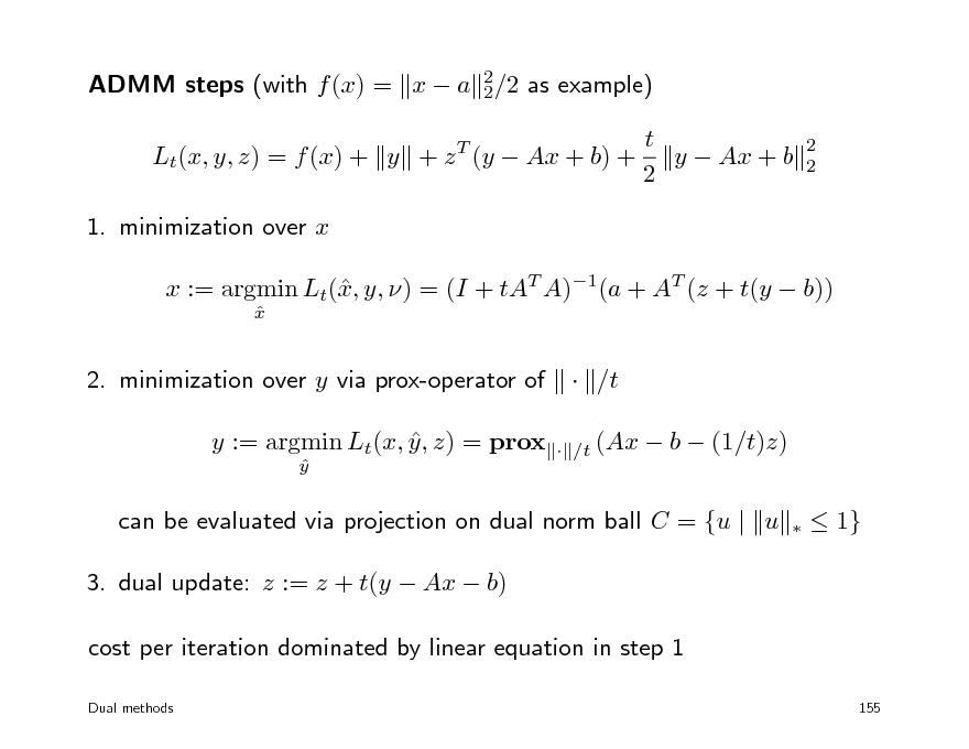
ADMM steps (with f (x) = x a 2/2 as example) 2 Lt(x, y, z) = f (x) + y + z T (y Ax + b) + 1. minimization over x x := argmin Lt(, y, ) = (I + tAT A)1(a + AT (z + t(y b)) x
x

t y Ax + b 2

2 2

2. minimization over y via prox-operator of y := argmin Lt(x, y , z) = prox
y

/t
/t (Ax

b (1/t)z)

can be evaluated via projection on dual norm ball C = {u | u 3. dual update: z := z + t(y Ax b) cost per iteration dominated by linear equation in step 1
Dual methods

1}

155

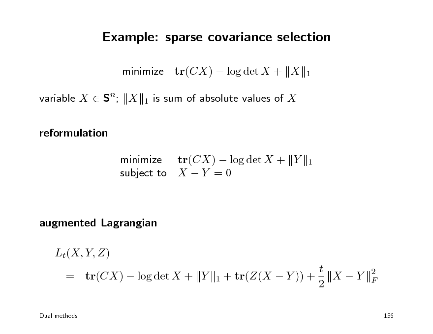
Example: sparse covariance selection
minimize tr(CX) log det X + X variable X Sn; X reformulation minimize tr(CX) log det X + Y subject to X Y = 0
1 1 1

is sum of absolute values of X

augmented Lagrangian Lt(X, Y, Z) t X Y = tr(CX) log det X + Y 1 + tr(Z(X Y )) + 2
Dual methods

2 F

156

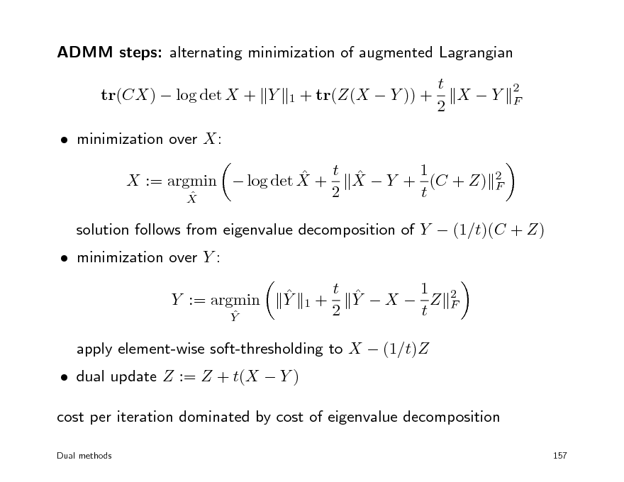
ADMM steps: alternating minimization of augmented Lagrangian tr(CX) log det X + Y minimization over X: t X Y + 1 (C + Z) X := argmin log det X + 2 t X
2 F 1 + tr(Z(X Y )) +

t X Y 2

2 F

minimization over Y :

solution follows from eigenvalue decomposition of Y (1/t)(C + Z) Y 1 t Y X Z 2 t
2 F

Y := argmin
Y

1+

dual update Z := Z + t(X Y )

apply element-wise soft-thresholding to X (1/t)Z

cost per iteration dominated by cost of eigenvalue decomposition
Dual methods 157

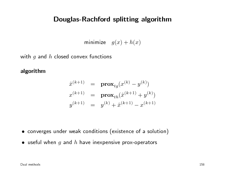
Douglas-Rachford splitting algorithm
minimize g(x) + h(x) with g and h closed convex functions algorithm x(k+1) = proxtg (x(k) y (k))

x(k+1) = proxth((k+1) + y (k)) x y (k+1) = y (k) + x(k+1) x(k+1)

converges under weak conditions (existence of a solution) useful when g and h have inexpensive prox-operators
Dual methods 158

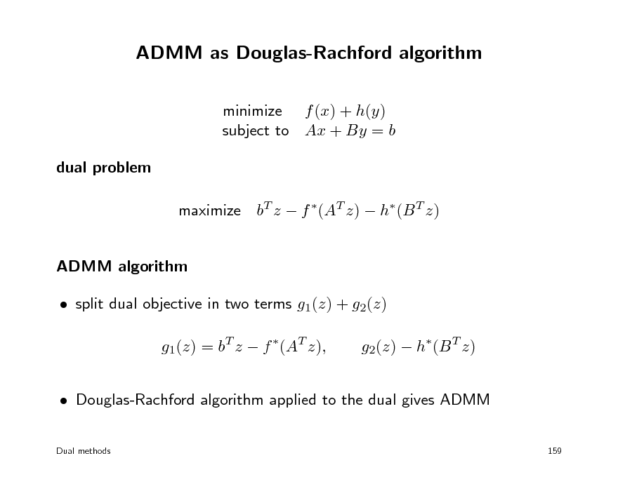
ADMM as Douglas-Rachford algorithm
minimize f (x) + h(y) subject to Ax + By = b dual problem maximize bT z f (AT z) h(B T z) ADMM algorithm split dual objective in two terms g1(z) + g2(z) g1(z) = bT z f (AT z), g2(z) h(B T z)

Douglas-Rachford algorithm applied to the dual gives ADMM
Dual methods 159

Sources and references
these lectures are based on the courses EE364A (S. Boyd, Stanford), EE236B (UCLA), Convex Optimization www.stanford.edu/class/ee364a www.ee.ucla.edu/ee236b/ EE236C (UCLA) Optimization Methods for Large-Scale Systems www.ee.ucla.edu/~vandenbe/ee236c EE364B (S. Boyd, Stanford University) Convex Optimization II www.stanford.edu/class/ee364b see the websites for expanded notes, references to literature and software

Dual methods

160