Understanding Neural Networks Through Deep Visualization
Quick links: ICML DL Workshop paper | code | video

These images are synthetically generated to maximally activate individual neurons in a Deep Neural Network (DNN). They show what each neuron “wants to see”, and thus what each neuron has learned to look for. The neurons selected for these images are the output neurons that a DNN uses to classify images as flamingos or school buses. Below we show that similar images can be made for all of the hidden neurons in a DNN. Our paper describes that the key to producing these images with optimization is a good natural image prior.
Background
Deep neural networks have recently been producing amazing results! But how do they do what they do? Historically, they have been thought of as “black boxes”, meaning that their inner workings were mysterious and inscrutable. Recently, we and others have started shinning light into these black boxes to better understand exactly what each neuron has learned and thus what computation it is performing.
Visualizing Neurons without Regularization/Priors
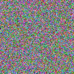
To visualize the function of a specific unit in a neural network, we synthesize inputs that cause that unit to have high activation. Here we will focus on images, but the approach could be used for any modality. The resulting synthetic image shows what the neuron “wants to see” or “what it is looking for”. This approach has been around for quite a while and was (re-)popularized by Erhan et al. in 2009. To synthesize such a “preferred input example”, we start with a random image, meaning we randomly choose a color for each pixel. The image will initially look like colored TV static:
Next, we do a forward pass using this image \(x\) as input to the network to compute the activation \(a_i(x)\) caused by \(x\) at some neuron \(i\) somewhere in the middle of the network. Then we do a backward pass (performing backprop) to compute the gradient of \(a_i(x)\) with respect to earlier activations in the network. At the end of the backward pass we are left with the gradient \(\partial a_i({x}) /\partial {x}\), or how to change the color of each pixel to increase the activation of neuron \(i\). We do exactly that by adding a little fraction \(\alpha\) of that gradient to the image:
\begin{align} x & \leftarrow x + \alpha \cdot \partial a_i({x}) /\partial {x} \end{align}
We keep doing that repeatedly until we have an image \(x^*\) that causes high activation of the neuron in question.
But what types of images does this process produce? As we showed in a previous paper titled Deep networks are easily fooled: high confidence predictions for unrecognizable images, the results when this process is carried out on final-layer output neurons are images that the DNN thinks with near certainty are everyday objects, but that are completely unrecognizable as such.

Synthesizing images without regularization leads to “fooling images”: The DNN is near-certain all of these images are examples of the listed classes (over 99.6% certainty for the class listed under the image), but they are clearly not. That’s because these images were synthesized by optimization to maximally activate class neurons, but with no natural image prior (e.g. regularization). Images are produced with gradient-based optimization (top) or two different, evolutionary optimization techniques (bottom). Images from Nguyen et al. 2014.
Visualizing Neurons with Weak Regularization/Priors
To produce more recognizable images, researchers have tried optimizing images to (1) maximally activate a neuron, and (2) have styles similar to natural images (e.g. not having pixels be at extreme values). These pressures for images to look like normal images are called “natural image priors” or “regularization.”
Simonyan et al. 2013 did this by adding L2-regularization to the optimization process, and in the resulting images one can start to recognize certain classes:

Images produced with weak regularization: These images are produced with the same gradient-ascent optimization technique mentioned above, but using only L2 regularization. Shown are images that light up the ImageNet “goose” and “ostrich” output neurons. From Simonyan et al. 2013.
Adding regularization thus helps, but it still tends to produce unnatural, difficult-to-recognize images. Instead of being comprised of clearly recognizable objects, they are composed primarily of “hacks” that happen to cause high activations: extreme pixel values, structured high frequency patterns, and copies of local motifs without global structure. In addition to Simonyan et al. 2013, Szegedy et al. 2013 showed optimized images of this type. Goodfellow et al. 2014 provided a great explanation for how such adversarial and fooling examples are to be expected due to the locally linear behavior of neural nets. In the supplementary section of our paper (linked at the top), we give one possible explanation for why gradient approaches tend to focus on high-frequency information.
Visualizing Neurons with Better Regularization/Priors
Our paper shows that optimizing synthetic images with better natural image priors produces even more recognizable visualizations. The figure at the top of this post showed some examples for ImageNet classes, and here is the full figure from the paper. You can also browse all fc8 visualizations on one page.

Synthetic images produced with our new, improved priors to cause high activations for different class output neurons (e.g. as tricycles and parking meters). The different types of images in each class represent different amounts of the four different regularizers we investigate in the paper. In the lower left are 9 visualizations each (in 3×3 grids) for four different sets of regularization hyperparameters for the Gorilla class. For all other classes, we have selected four interpretable examples. For example, the lower left quadrant tends to show lower frequency patterns, the upper right shows high frequency patterns, and the upper left shows a sparse set of important regions. Often greater intuition can be gleaned by considering all four at once. In many cases we have found that one can guess what class a neuron represents by viewing sets of these optimized, preferred images. You can browse all fc8 visualizations here.
How are these figures produced? Specifically, we found four forms of regularization that, when combined, produce more recognizable, optimization-based samples than previous methods. Because the optimization is stochastic, by starting at different random initial images, we can produce a set of optimized images whose variance provides information about the invariances learned by the unit. As a simple example, we can see that the pelican neuron will fire whether there are two pelicans or only one.
Visualizing Neurons from All Layers
These images can be produced for any neuron in the DNN, including hidden neurons. Doing so sheds light on which features have been learned at each layer, which helps us both to understand how current DNNs work and to fuels intuitions for how to improve them. Here are example images from all layers of a network similar to the famous AlexNet from Krizhevsky et al, 2012.

All Layers: Images that light up example features of all eight layers on a network similar to AlexNet. The images reflect the true sizes of the features at different layers. For each feature in each layer, we show visualizations from 4 random gradient descent runs. One can recognize important features at different scales, such as edges, corners, wheels, eyes, shoulders, faces, handles, bottles, etc. Complexity increases in higher-layer features as they combine simpler features from lower layers. The variation of patterns also increases in higher layers, revealing that increasingly invariant, abstract representations are learned. In particular, the jump from Layer 5 (the last convolution layer) to Layer 6 (the first fully-connected layer) brings about a large increase in variation. Click on the image to zoom in.
Putting it together: the Deep Visualization Toolbox
Our paper describes a new, open source software tool that lets you probe DNNs by feeding them an image (or a live webcam feed) and watching the reaction of every neuron. You can also select individual neurons to view pre-rendered visualizations of what that neuron “wants to see most”. We’ve also included deconvolutional visualizations produced by Zeiler and Fergus (2014) that show which pixels in an image cause that neuron to activate. Finally, we include the image patches from the training set that maximally light up that image.
In short, we’ve gathered a few different methods that allow you to “triangulate” what feature a neuron has learned, which can help you better understand how DNNs work.
Video tour of the Deep Visualization Toolbox. Best in HD!
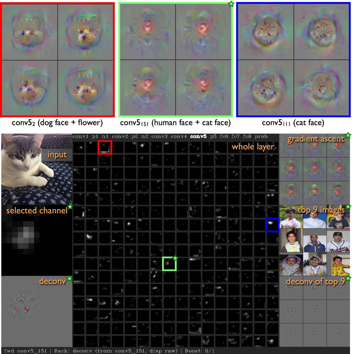
Screenshot of the Deep Visualization Toolbox when processing Ms. Freckles’ regal face. The above video provides a description of the information shown in each region.
Why does this matter?
Interacting with DNNs can teach us a few things about how they work. These interactions can help build our intuitions, which can in turn help us design better models. So far the visualizations and toolbox have taught us a few things:
- Important features such as face detectors and text detectors are learned, even though we do not ask the networks to specifically learn these things. Instead, it learns them because they help with other tasks (e.g. identifying bowties, which are usually paired with faces, and bookcases, which are usually full of books labeled with text).
- Some have supposed that DNN representations are highly distributed, and thus any individual neuron or dimension is uninterpretable. Our visualizations suggest that many neurons represent abstract features (e.g. faces, wheels, text, etc.) in a more local — and thus interpretable — manner.
- It was thought, and even we have argued, that supervised discriminative DNNs ignore many aspects of objects (e.g. the outline of a starfish and the fact that it has five legs) and instead only key on the one or few unique things that make it possible to identify that object (e.g. the rough, orange texture of a starfish’s skin). Instead, these new, synthetic images show that discriminatively trained networks do in fact learn much more than we thought, including much about the global structure of objects. For more discussion on this issue, see the last two paragraphs of our paper.
This last observation raises some interesting possible security concerns. For example, imagine you own a phone or personal robot that cleans your house, and in the phone or robot is a DNN that learns from its environment. Imagine that, to preserve your privacy, the phone or robot does not explicitly store any pictures or videos obtained during operation, but they do use visual input to train their internal network to better perform their tasks. The above results show that given only the learned network, one may still be able to reconstruct things that you would not want released, such as pictures of your valuables, or your bedroom, or videos of what you do when you are home alone, such as walking around naked singing Somewhere Over the Rainbow.
How does this relate to...
... Mahendran and Vedaldi (2014)?
Mahendran and Vedaldi (2014) showed the importance of incorporating natural-image priors in the optimization process. Like Zeiler and Fergus, their method starts from a specific input image. They record the network’s representation of that specific image and then reconstruct an image that produces a similar code. Thus, their method provides insight into what the activation of a whole layer represent, not what an individual neuron represents. This is a very useful and complementary approach to ours in understanding how DNNs work.
... Google's “Inceptionism” (aka #DeepDream)?
To produce their single-class images, the Inceptionism team uses the same gradient ascent technique employed here and in other works (Erhan et al. 2009). They also build on the idea in our paper and in Mahendran and Vedaldi (2014) that stronger natural image priors are necessary to produce better visualizations with this gradient ascent technique. Their prior that "neighboring pixels be correlated" is similar both to one of our priors (Gaussian blur) and to Mahendran and Vedaldi's minimization of “total variation”, emphasizing the likely importance of these sorts of priors in the future!
... Zeiler and Fergus’ “Deconvolutional” networks?
The deconvnet technique is quite different. Like Mahendran and Vedaldi, the deconv visualizations of Zeiler and Fergus (2014) are produced beginning with an input image, as opposed to beginning with a sample of noise. Their method then highlights which pixels in that image contributed to a neuron firing, but in a slightly different (and more interpretable) manner than using straight backprop. This is another very useful and complementary method that provides different insights about neural networks when applied to specific images.
Resources
- ICML DL Workshop paper
- Deep Visualization Toolbox code on github (also fetches the below resources)
- Caffe network weights (223M) for the caffenet-yos model used in the video and for computing visualizations.
-
Pre-computed per-unit visualizations (“123458” = conv1-conv5 and fc8. “67” = fc6 and fc7.)
Regularized opt: 123458 (449M), 67 (2.3G)
Max images: 123458 (367M), 67 (1.3G)
Max deconv: 123458 (267M), 67 (981M).
Thanks for your interest. Try it out for yourself
and let us know what you find!
— Jason, Jeff, Anh, Thomas, and Hod
Posted June 26, 2015. Updated July 8, 2015.