Kernel Methods for Statistical Learning
Kenji Fukumizu
The Institute of Statistical Mathematics / Graduate University for Advanced Studies September 6-7, 2012 Machine Learning Summer School 2012, Kyoto Version 2012.09.04 The latest version of slides is downloadable at http://www.ism.ac.jp/~fukumizu/MLSS2012/

1

Lecture Plan
I. Introduction to kernel methods
kernel PCA, kernel CCA, kernel ridge regression, etc A brief introduction to SVM

II. Various kernel methods

III. Support vector machine IV. Theoretical backgrounds of kernel methods
Mathematical aspects of positive definite kernels Recent advances of kernel methods

V. Nonparametric inference with positive definite kernels

2

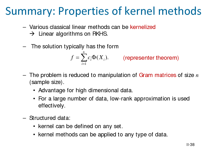
General references
each section)

(More detailed lists are given at the end of

Schlkopf, B. and A. Smola. Learning with Kernels. MIT Press. 2002. Lecture slides (more detailed than this course) This page contains Japanese information, but the slides are written in English. Slides: 1, 2, 3, 4, 5, 6, 7, 8 For Japanese only (Sorry!): 2010 2008

3

I. Introduction to Kernel Methods
Kenji Fukumizu
The Institute of Statistical Mathematics / Graduate University for Advanced Studies September 6-7 Machine Learning Summer School 2012, Kyoto
I-1 1

Outline
1. Linear and nonlinear data analysis 2. Principles of kernel methods 3. Positive definite kernels and feature spaces

I-2 2

LinearandNonlinearDataAnalysis

I-3 3

Whatisdataanalysis?
Analysis of data is a process of inspecting, cleaning, transforming, and modeling data with the goal of highlighting useful information, suggesting conclusions, and supporting decision making. Wikipedia

I-4

Lineardataanalysis
Table of numbers Matrix expression
( X 1(1) X m1) ( X 1( 2 ) X m2 ) X X (N ) X (N ) m 1

m dimensional, N data

Linear algebra is used for methods of analysis Correlation, Linear regression analysis, Principal component analysis, Canonical correlation analysis, etc.
I-5

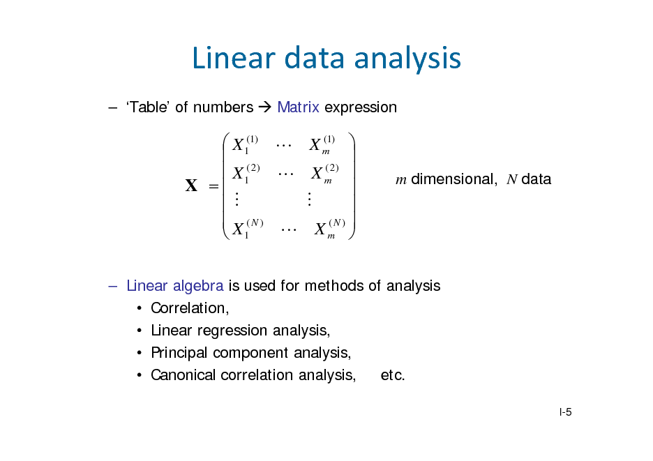
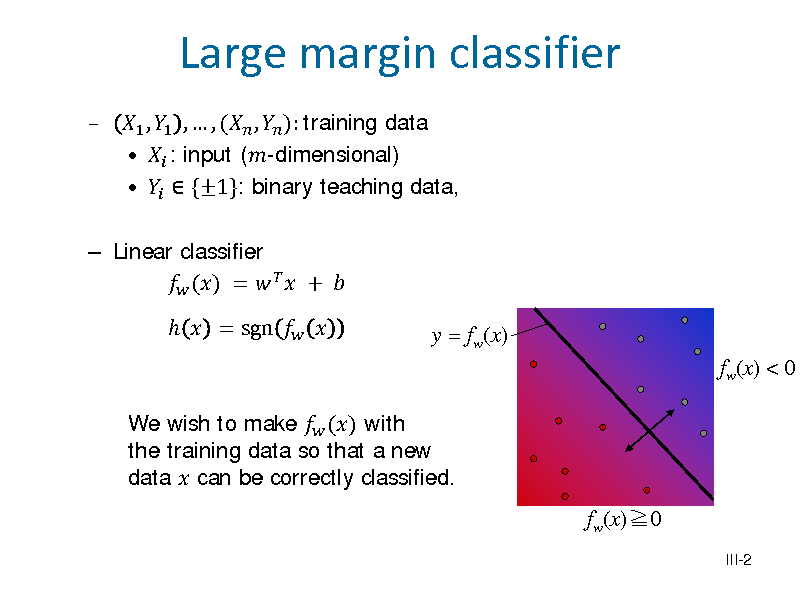
Example 1: Principal component analysis (PCA)
PCA: project data onto the subspace with largest variance. 1st direction =

argmax ||a||1Var[a T X ]
Var[a T X ] T (i ) 1 a X N i 1 a T VXX a. 1 N
N

X ( j ) j 1
N

2

where
1 VXX N (i ) 1 X N i 1
N

1 X ( j ) X ( i ) j 1 N
N

X ( j) j 1
N

T

(Empirical) covariance matrix of
I-6

1st principal direction

argmax||a||1a T VXX a
u1
unit eigenvector w.r.t. the largest eigenvalue of

p-th principal direction = unit eigenvector w.r.t. the p-th largest eigenvalue of

PCA

Eigenproblem of covariance matrix

I-7

Example 2: Linear classification
Binary classification Input data
( X 1(1) X m1) ( 2) ( 2) X Xm X 1 X (N ) X (N ) m 1

Class label

Y (1) ( 2) Y {1}N Y Y ( N )

Find a linear classifier

h( x ) sgn(a T x b)
so that

h( X ( i ) ) Y ( i )

for all (or most) i.

Example: Fishers linear discriminant analyzer, Linear SVM, etc.
I-8

Arelinearmethodsenough?
linearly inseparable
6

linearly separable
15 10 5

4

2

z3 x2
0

0 -5

transform

-10 -15 0 5 20 10 10 15 20 0 5 15

-2

-4

-6 -6

z1
-4 -2 0 2 4 6

x1
2 ( z1 , z 2 , z3 ) ( x12 , x2 , 2 x1 x2 )

z2

Watch the following movie! http://jp.youtube.com/watch?v=3liCbRZPrZA

I-9

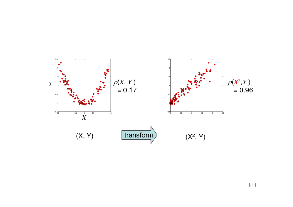
Another example: correlation
XY
Cov[ X , Y ] E X E[ X ]Y E[Y ] 2 2 Var[ X ]Var[Y ] E X E[ X ] E Y E[Y ]

3

2

= 0.94

1

Y

0

-1

-2

-3 -3

-2

-1

0

1

2

3

X
I-10

2.5

2.5

2

2

1.5

Y

1

(X, Y )
= 0.17

1.5

1

(X2,Y )
= 0.96

0.5

0.5

0

0

-0.5 -1.5

-1

-0.5

0

0.5

1

1.5

-0.5 0

0.5

1

1.5

2

2.5

X (X, Y) transform (X2, Y)

I-11

Nonlineartransformhelps!
Analysis of data is a process of inspecting, cleaning, transforming, and modeling data with the goal of highlighting useful information, suggesting conclusions, and supporting decision making.

Wikipedia.

Kernel method = a systematic way of transforming data into a highdimensional feature space to extract nonlinearity or higher-order moments of data.

I-12

Principlesofkernelmethods

I-13

Kernelmethod:Bigpicture
Idea of kernel method feature map
x
i

x Space of original data

xi

x

Hk
j

,

Feature space Do linear analysis in the feature space! e.g. SVM

What kind of space is appropriate as a feature space? Should incorporate various nonlinear information of the original data. The inner product should be computable. It is essential for many linear methods.
I-14

Computational issue
For example, how about using power series expansion? (X, Y, Z) (X, Y, Z, X2, Y2, Z2, XY, YZ, ZX, ) But, many recent data are high-dimensional. e.g. microarray, images, etc... The above expansion is intractable! e.g. Up to 2nd moments, 10,000 dimension: Dim of feature space: Need a cleverer way
10000C1

+

10000C2

= 50,005,000 (!)

Kernel method.

I-15

Featurespacebypositivedefinitekernel
Feature map: from original space to feature space

: H X 1 ,, X n
( X 1 ),, ( X n )

With special choice of feature space, we have a function (positive definite kernel) k(x, y) such that

( X i ), ( X j ) k ( X i , X j )

kernel trick.

Many linear methods use only the inner products of data, and do not need the explicit form of the vector . (e.g. PCA)
I-16

Positivedefinitekernel
Definition. : set. : is a positive definite kernel if 1) (symmetry)

k ( x, y ) k ( y , x )

2) (positivity) for arbitrary x1, , xn

k ( x1 , x1 ) k ( x1 , xn ) k(x , x ) k(x , x ) n 1 n n
(Gram matrix) i.e.,

is positive semidefinite,

n

i , j 1 i

c c j k ( xi , x j ) 0

for any

ci R

I-17

Examples: positive definite kernels on Rm (proof is give in Section IV) Euclidean inner product

k ( x, y ) x T y
Gaussian RBF kernel

kG ( x, y ) exp x y
Laplacian kernel

2

2

( 0)

k L ( x, y ) exp i 1 | xi yi |
m

( 0)

Polynomial kernel

k P ( x, y ) ( c x T y ) d

( c 0, d N )
I-18

Proposition 1.1 Let be a vector space with inner product , and : be a map (feature map). If : is defined by

( x ), ( y ) k ( x, y ),
then k(x,y) is necessarily positive definite. Positive definiteness is necessary. Proof)

I-19

Positive definite kernel is sufficient. Theorem 1.2 (Moore-Aronszajn) For a positive definite kernel on , there is a Hilbert space (reproducing kernel Hilbert space, RKHS) that consists of functions on such that 1) , for any 2) span , is dense in 3) (reproducing property)

,

,

for any

,

*Hilbert space: vector space with inner product such that the topology is complete.

I-20

Featuremapbypositivedefinite kernel
Feature space = RKHS. Feature map:

: ,,

, ,

,,

, ,

Kernel trick: by reproducing property

,

,

,

,

,

Prepare only positive definite kernel: We do not need an explicit form of feature vector or feature space. All we need for kernel methods are kernel values , .
I-21

II. Various Kernel Methods
Kenji Fukumizu
The Institute of Statistical Mathematics / Graduate University for Advanced Studies September 6-7 Machine Learning Summer School 2012, Kyoto
1

Outline
1. Kernel PCA 2. Kernel CCA 3. Kernel ridge regression 4. Some topics on kernel methods

II-2

Kernel Principal Component Analysis

II-3

Principal Component Analysis
PCA (review)
Linear method for dimension reduction of data Project the data in the directions of large variance. 1st principal axis = argmax||a|| =1Var[ a X ]
T

1 n T 1 n T Var[a X ] = a X i j =1 X j n i =1 n
= a T VXX a.
where
1 n 1 n 1 n = X i j =1 X j X i j =1 X j n i =1 n n
T

2

VXX

II-4

From PCA to Kernel PCA
Kernel PCA: nonlinear dimension reduction of data 1998). Do PCA in feature space
(Schlkopf et al.

max ||a||=1 :

Var[a T X ] =

1 T 1 n a X i s =1 X s n i =1 n
n

2

max || f ||H =1 : Var[ f , ( X ) ] =

1 1 n f , ( X i ) s =1 ( X s ) n i =1 n
n

2

II-5

It is sufficient to assume

Orthogonal directions to the data can be neglected, since for 1 = ( ) + , where is orthogonal to =1 =1 }=1, the objective function of kernel the span{ PCA does not depend on .
1 =1

=
=1

1
=1

Then,

~2 Var[ f , ( X ) ] = cT K X c 2 T ~ || f ||H = c K X c

[Exercise] (centered Gram matrix)

~ ~ ~ where K X , ij := ( X i ), ( X j )
with

n ~ 1 ( X i ) := ( X i ) n s =1 ( X s )

(centered feature vector)
II-6

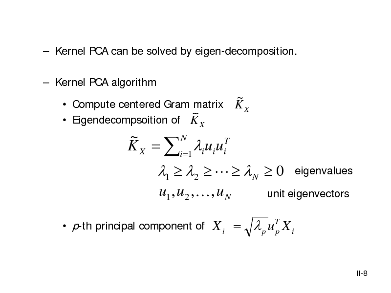
Objective function of kernel PCA
~2 max c K X c
T

subject to

~ c KX c = 1
T

The centered Gram matrix is expressed with Gram matrix = , as 1 =

1 n = k ( X i , X j ) s =1 k ( X i , X s ) ij n 1 n 1 t =1 k ( X t , X j ) + 2 n n [Exercise] ~ KX

( )

1

1 = 1

N

= Unit matrix

t , s =1

k( Xt , X s )
II-7

Kernel PCA can be solved by eigen-decomposition. Kernel PCA algorithm Compute centered Gram matrix ~ Eigendecompsoition of K X
N ~ K X = i =1 i ui uiT

~ KX

1 2 N 0
u1 , u2 , , u N
p-th principal component of

eigenvalues

unit eigenvectors

X i = p uT X i p

II-8

Derivation of kernel method in general
Consider feature vectors with kernels. Linear method is applied to the feature vectors. (Kernelization) Typically, only the inner products

( X i ), ( X j ) = k ( X i , X j )
f , ( X i )
are used to express the objective function of the method. The solution is given in the form
n

f = ci ( X i ),
i =1

(representer theorem, see Sec.IV), and thus everything is written by Gram matrices. These are common in derivation of any kernel methods.
II-9

Example of Kernel PCA
Wine data
(from UCI repository)

13 dim. chemical measurements of for three types of wine. 178 data. Class labels are NOT used in PCA, but shown in the figures. First two principal components:
4

Linear PCA

0.6

Kernel PCA (Gaussian kernel) ( = 3)

3

0.4

2

0.2
1

0
0

-0.2
-1

-2

-0.4

-3

-0.6

-4 -5

0

5

-0.8 -0.8

-0.6

-0.4

-0.2

0

0.2

0.4

0.6

II-10

Kernel PCA (Gaussian)
0.5 0.4 0.3 0.2 0.1 0 -0.1 -0.2 -0.3

=2

0.6

=4

0.4

0.2

0

-0.2

-0.4

-0.6
-0.4 -0.5 -0.5

-0.4

-0.3

-0.2

-0.1

0

0.1

0.2

0.3

0.4

-0.8 -0.8

-0.6

-0.4

-0.2

0

0.2

0.4

0.6

0.6

=5

0.4

0.2

0

kG ( x, y ) = exp x y

(

2

2

)

-0.2

-0.4

-0.6

-0.8 -0.8

II-11
-0.6 -0.4 -0.2 0 0.2 0.4 0.6

Noise Reduction with Kernel PCA
PCA can be used for noise reduction (principal directions represent signal, other directions noise). Apply kernel PCA for noise reduction: Compute d-dim subspace Vd spanned by d-principal directions. For a new data x, Gx: Projection of (x) onto Vd = noise reduced feacure vector. Compute a preimage x in data sapce for the noise (x) reduced feature vector Gx. Gx 2
10 8 6

x = arg min ( x) Gx
x

4 2 0

-2

Note: Gx is not necessariy given as an image of .

-4 -6 -8 0 -10 -25 -20 -15 -10 -5 0 5 10 15 20 20 -20

II-12

USPS data

Original data (NOT used for PCA)

Noisy images

Noise reduced imageslinear PCA

Noise reduced images kernel PCA, Gaussian kernel Generated by Matlab stprtool (by V. Franc)
II-13

Properties of Kernel PCA
Nonlinear features can be extracted. Can be used for a preprocessing of other analysis like classification. (dimension reduction / feature extraction) The results depend on the choice of kernel and kernel parameters. Interpreting the results may not be straightforward. How to choose a kernel and kernel parameter? Cross-validation is not straightforward unlike SVM. If it is a preprocessing, the performance of the final analysis should be maximized.

II-14

Kernel Canonical Correlation Analysis

II-15

Canonical Correlation Analysis
Canonical correlation analysis (CCA, Hotelling 1936) Linear dependence of two multivariate random vectors. Data 1 , 1 , , ( , ) : m-dimensional, : -dimensional

Find the directions and so that the correlation of and is maximized.

= max Corr[a X , b Y ] = max
T T a ,b a ,b

Cov[a T X , bT Y ]
T

Var[a X ]Var[b Y ]

T

,

a X

a TX

b TY

b Y
II-16

Solution of CCA
,

Rewritten as a generalized eigenproblem:

max

subject to

[Exercise: derive this. (Hint. Use Lagrange multiplier method.)] Solution: = 1 , = 1
1/2 1/2

=

= = 1.

where 1 (1 , resp.) is the left (right, resp.) first eigenvector 1/2 1/2 . for the SVD of
II-17

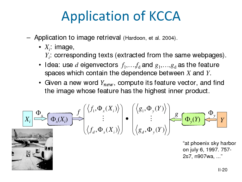
Kernel CCA
Kernel CCA (Akaho 2000, Melzer et al. 2002, Bach et al 2002) Dependence (not only correlation) of two random variables. Data: 1 , 1 , , ( , ) arbitrary variables Consider CCA for the feature vectors with and : 1 , , 1 , , , , 1 , , 1 , , .
max Var Var[ ] Cov[ , ] =
,

,

max

,

, ,
2

,

2

X

x

x(X)

f

f (X )

g (Y )

g

y(Y)

y

Y
II-18

We can assume = ( ) and = ( ). =1 =1 maxR, 2 2
2

and : centered Gram matrices.

(same as kernel PCA)

Regularization: to avoid trivial solution,
,

max

Solution: generalized eigenproblem

, =1

, , =1 2 + = +
2

, =1

2

2 +

+

2

II-19

Application of KCCA
Application to image retrieval (Hardoon, et al. 2004). Xi: image, Yi: corresponding texts (extracted from the same webpages). Idea: use d eigenvectors f1,,fd and g1,,gd as the feature spaces which contain the dependence between X and Y. Given a new word , compute its feature vector, and find the image whose feature has the highest inner product. Xi x x(Xi) f

f1 , x ( X i ) f , (X ) d x i

g1 , y (Y ) g , (Y ) d y

g y(Y)

y

Y

at phoenix sky harbor on july 6, 1997. 7572s7, n907wa, ...
II-20

Example: Gaussian kernel for images. Bag-of-words kernel (frequency of words) for texts. Text -- height: 6-11, weight: 235 lbs, position: forward, born: september 18, 1968, split, croatia college: none Extracted images

II-21

Kernel Ridge Regression

II-22

1 , 1 , , , : data ( , ) Ridge regression: linear regression with 2 penalty. min |2 |2 +
=1 2

Ridge regression

(The constant term is omitted for simplicity)

Solution (quadratic function): = + 1 where =
1 , 1 =

Ridge regression is preferred, when is (close to) singular.

1 , =

II-23

1 , 1 , , , : arbitrary data, . Kernelization of ridge regression: positive definite kernel for equivalently, min | ,
=1 =1

Kernel ridge regression
| 2

min | ( )|2 +

+

2

2

Ridge regression on Nonlinear ridge regr.

II-24

Solution is given by the form

Objective function :

Let = + = + =1 ( , : orthogonal complement) =1 Objective function = =1 + , 2 + + 2 = , 2 + ( 2 + 2 ) =1 The 1st term does not depend on , and 2nd term is minimized in the case = 0.
j =1

f = c j ( X j ),

n

Solution: = + Function: =

1

2

+

+
1

, 1 = ,

II-25

Regularization
The minimization may be attained with zero errors. But the function may not be unique. Regularization

min

2

Regularization with smoothness penalty is preferred for uniqueness and smoothness. Link with some RKHS norm and smoothness is discussed in Sec. IV.

min | ( )|2 + =1

2

II-26

Comparison
Kernel ridge regression vs local linear regression
= 100, 500 runs
2

= 1/ 1.5 + | |

+ ,

0.012 0.01

~ 0, , ~ 0, 0.12

Kernel method Local linear

Mean square errors

Kernel ridge regression with Gaussian kernel Local linear regression with Epanechnikov kernel (locfit in R is used) Bandwidth parameters are chosen by CV.

0.008 0.006 0.004 0.002 0 1

10 Dimension of X

100
II-27

Local linear regression

: smoothing kernel ( 0, = 1, not necessarily positive definite)
(e.g., Fan and Gijbels 1996)

Local linear regression = 0 is estimated by
,

For each 0 , this minimization can be solved by linear algebra. Statistical property of this estimator is well studied. For one dimensional , it works nicely with some theoretical optimality. But, weak for high-dimensional data.
II-28

min ( 0 ) 2 ( 0 )

() =

Some topics on kernel methods
Representer theorem Structured data Kernel choice Low rank approximation

II-29

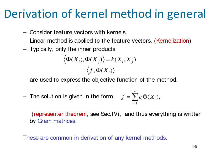
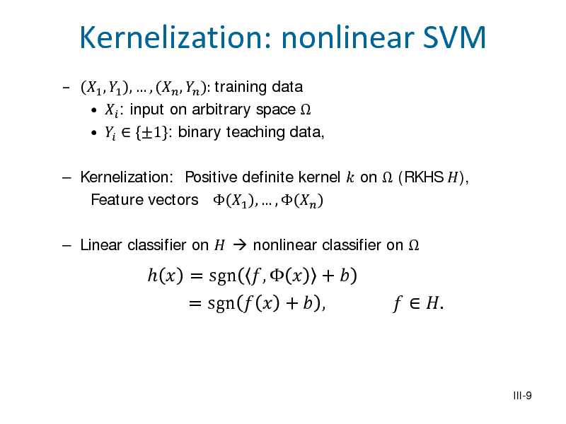
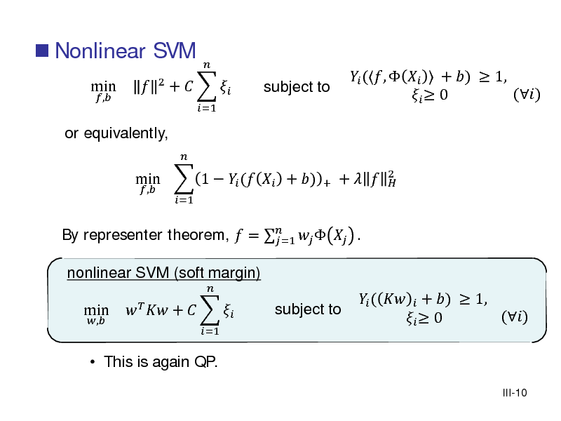
1 , 1 , , , : data : positive definite kernel for , : corresponding RKHS. : monotonically increasing function on + . Theorem 2.1 (representer theorem, Kimeldorf & Wahba 1970) The solution to the minimization problem: is attained by = =1

Representer theorem

min (1 , 1 , 1 , , ( , , )) + (| |)

The proof is essentially the same as the one for the kernel ridge regression. [Exercise: complete the proof]
II-30

with some 1 , , .

Structured Data
Structured data: non-vectorial data with some structure. Sequence data (variable length): DNA sequence, Protein (sequence of amino acid) Text (sequence of words) Graph data (Kojis lecture) Chemical compound etc. Tree data Parse tree Histograms / probability measures NP S VP NP Det The N V Det N

cat chased the mouse.
(Haussler 1999).
II-31

Many kernels uses counts of substructures

Spectrum kernel
p-spectrum kernel Example: s = statistics 3-spectrum
s: sta, tat, ati, tis, ist, sti, tic, ics t : pas, ast, sta, tap, api, pis, ist, sta, tan
sta (s) (t) 1 2 tat 1 0 ati 1 0 tis 1 0 ist 1 1 sti 1 0 tic 1 0 ics 1 0 pas 0 1 ast 0 1 tap 0 1 api 0 1 pis 0 1 tan 0 1

, = Occurrences of common subsequences of length p.
(Leslie et al 2002):

positive definite kernel for string.

t = pastapistan

Linear time (((|| + ||) ) algorithm with suffix tree is known II-32 (Vishwanathan & Smola 2003).

K3(s, t) 12 + 11 = 3

Application: kernel PCA of words with 3-spectrum kernel
8 bioinformatics 6 informatics 4 2 mathematics biology psychology cybernetics 0 physics methodology -2 -4 -6 -4 pioneering engineering metaphysics

statistics biostatistics

-2

0

2

4

6

8

II-33

Choice of kernel
Choice of kernel
Choice of kernel (polyn or Gauss) Choice of parameters (bandwidth parameter in Gaussian kernel)

General principles
Reflect the structure of data (e.g., kernels for structured data) For supervised learning (e.g., SVM) Cross-validation For unsupervised learning (e.g. kernel PCA) No general methods exist. Guideline: make or use a relevant supervised problem, and use CV. Learning a kernel: Multiple kernel learning (MKL) , = (, ) optimize =1

II-34

Gram matrix: where is the sample size. Large causes computational problems. e.g. Inversion, eigendecomposition costs (3 ) in time. Low-rank approximation

Low rank approximation
,

where : matrix ( < )

The decay of eigenvalues of a Gram matrix is often quite fast (See Widom 1963, 1964; Bach & Jordan 2002).
II-35

Two major methods Incomplete Cholesky factorization (Fine & Sheinberg 2001) ( 2 ) in time and () in space Nystrm approximation (Williams and Seeger 2001) Random sampling + eigendecomposition Example: kernel ridge regression +
1

Low rank approximation: . With Woodbury formula*
1

+

+ =
1

+

time : (3 )
1

* Woodbury (ShermanMorrisonWoodbury) formula: + 1 = 1 1 + 1 1 1 .

time : ( 2 + 3 )

1

II-36

Other kernel methods
Kernel Fisher discriminant analysis kernel FDA
(Mika et al. 1999)

Kernel logistic regression Roth 2001, Zhu&Hastie 2005 Kernel partial least squarekernel PLSRosipal&Trejo 2001 Kernel K-means clusteringDhillon et al 2004 etc, etc, ... Variants of SVM Section III.

II-37

Summary: Properties of kernel methods
Various classical linear methods can be kernelized Linear algorithms on RKHS. The solution typically has the form
n

f = ci ( X i ).
i =1

(representer theorem)

The problem is reduced to manipulation of Gram matrices of size n (sample size). Advantage for high dimensional data. For a large number of data, low-rank approximation is used effectively. Structured data: kernel can be defined on any set. kernel methods can be applied to any type of data.
II-38

References
Akaho. (2000) Kernel Canonical Correlation Analysis. Proc. 3rd Workshop on Induction-based Information Sciences (IBIS2000). (in Japanese) Bach, F.R. and M.I. Jordan. (2002) Kernel independent component analysis. Journal of Machine Learning Research, 3:148. Dhillon, I. S., Y. Guan, and B. Kulis. (2004) Kernel k-means, spectral clustering and normalized cuts. Proc. 10th ACM SIGKDD Intern. Conf. Knowledge Discovery and Data Mining (KDD), 551556. Fan, J. and I. Gijbels. Local Polynomial Modelling and Its Applications. Chapman Hall/CRC, 1996. Fine, S. and K. Scheinberg. (2001) Efficient SVM Training Using Low-Rank Kernel Representations. Journal of Machine Learning Research, 2:243-264. Gkhan, B., T. Hofmann, B. Schlkopf, A.J. Smola, B. Taskar, S.V.N. Vishwanathan. (2007) Predicting Structured Data. MIT Press. Hardoon, D.R., S. Szedmak, and J. Shawe-Taylor. (2004) Canonical correlation analysis: An overview with application to learning methods. Neural Computation, 16:2639 2664. Haussler, D. Convolution kernels on discrete structures. Tech Report UCSC-CRL-99-10, Department of Computer Science, University of California at Santa Cruz, 1999.
II-39

Leslie, C., E. Eskin, and W.S. Noble. (2002) The spectrum kernel: A string kernel for SVM protein classification, in Proc. Pacific Symposium on Biocomputing, 564575. Melzer, T., M. Reiter, and H. Bischof. (2001) Nonlinear feature extraction using generalized canonical correlation analysis. Proc. Intern. Conf. .Artificial Neural Networks (ICANN 2001), 353360. Mika, S., G. Rtsch, J. Weston, B. Schlkopf, and K.-R. Mller. (1999) Fisher discriminant analysis with kernels. In Y.-H. Hu, J. Larsen, E. Wilson, and S. Douglas, edits, Neural Networks for Signal Processing, volume IX, 4148. IEEE. Rosipal, R. and L.J. Trejo. (2001) Kernel partial least squares regression in reproducing kernel Hilbert space. Journal of Machine Learning Research, 2: 97123. Roth, V. (2001) Probabilistic discriminative kernel classifiers for multi-class problems. In Pattern Recognition: Proc. 23rd DAGM Symposium, 246253. Springer. Schlkopf, B., A. Smola, and K-R. Mller. (1998) Nonlinear component analysis as a kernel eigenvalue problem. Neural Computation, 10:12991319. Schlkopf, B. and A. Smola. Learning with Kernels. MIT Press. 2002. Vishwanathan, S. V. N. and A.J. Smola. (2003) Fast kernels for string and tree matching. Advances in Neural Information Processing Systems 15, 569576. MIT Press. Williams, C. K. I. and M. Seeger. (2001) Using the Nystrm method to speed up kernel machines. Advances in Neural Information Processing Systems, 13:682688.
II-40

Widom, H. (1963) Asymptotic behavior of the eigenvalues of certain integral equations. Transactions of the American Mathematical Society, 109:278{295, 1963. Widom, H. (1964) Asymptotic behavior of the eigenvalues of certain integral equations II. Archive for Rational Mechanics and Analysis, 17:215{229, 1964.

II-41

Appendix

II-42

Exercise for kernel PCA
~ || f ||2 = cT K X c H

2

= ,
=1

2 Var f , ( X ) = cT K X c

[

Var ,

]

=1

= ,
2

= .

~

=

1 = , =
=1 =1 =1

1 ,
=1 =1

1 1 2 =

=1

,

II-43

III. Support Vector Machines
A Brief Introduction Kenji Fukumizu
The Institute of Statistical Mathematics / Graduate University for Advanced Studies September 6-7 Machine Learning Summer School 2012, Kyoto
1

Linear classifier () = + = sgn

1 , 1 , , ( , ): training data : input (-dimensional) {1}: binary teaching data,

Large margin classifier

y = fw(x) fw(x) < 0

We wish to make () with the training data so that a new data can be correctly classified.

fw(x)0
III-2

Large margin criterion
Assumption: the data is linearly separable. Among infinite number of separating hyperplanes, choose the one to give the largest margin. Margin = distance of two classes measured along the direction of .
8 6 4

Support vector machine: Hyperplane to give the largest margin. The classifier is the middle of the margin. Supporting points on the two boundaries are called support vectors.

2

support vector

0

-2

-4

-6

margin
-6 -4 -2 0 2 4 6 8

-8 -8

III-3

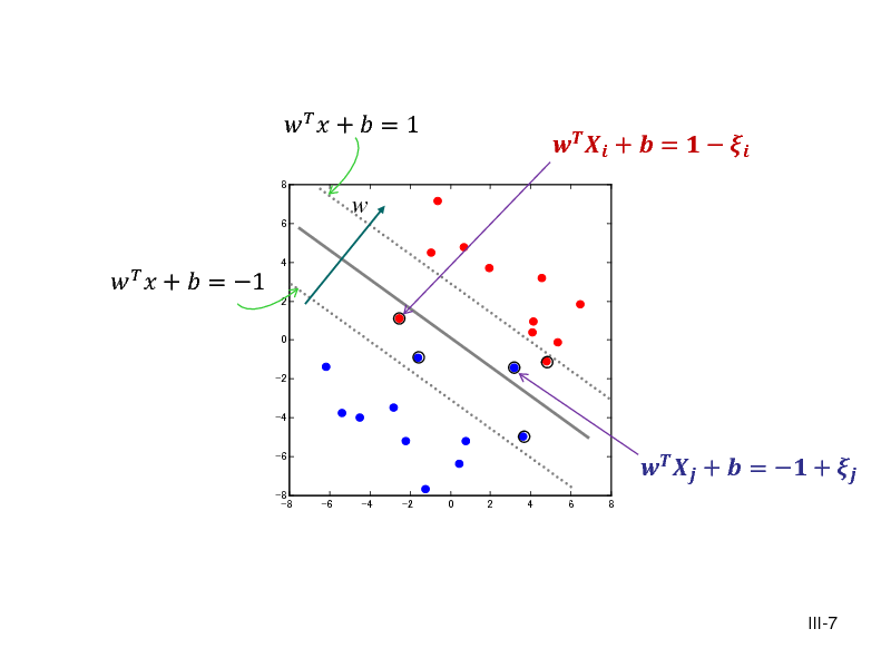
Fix the scale (rescaling of (, ) does not change the plane) Then

min( wT X i + b) = 1 if Yi = 1, max( wT X i + b) = 1 if Yi = 1
2 Margin =

[Exercise] Prove this.

III-4

Support vector machine (linear, hard margin)
(Boser, Guyon, Vapnik 1992)

Objective function: max
,

1

+ 1 if = 1, subject to + 1 if = 1. ( + ) 1 ()

SVM (hard margin)
,

Quadratic program (QP): Minimization of a quadratic function with linear constraints. Convex, no local optima (Vandenberghe lecture) Many solvers available (Chih-Jen Lins lecture)
III-5

min

2

subject to

Soft-margin SVM
Linear separability is too strong. Relax it. ( + ) 1
,

Hard margin

SVM (soft margin)

min

2

+

=1

( + ) 1 , subject to

Soft margin

( + ) 1 , 0 ()

0

This is also QP. The coefficient C must be given. Cross-validation is often used.

III-6

8

+ = 1 w

+ = 1

+ =

6

4

2

0

-2

-4

-6

-8 -8

-6

-4

-2

0

2

4

6

8

+ = +

III-7

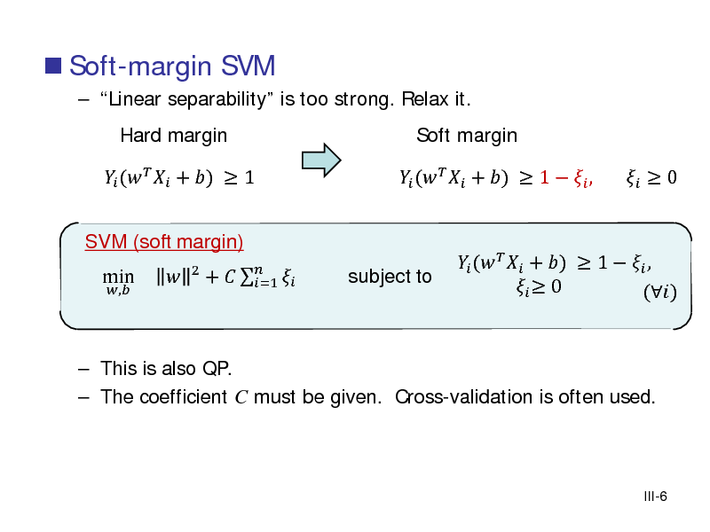
SVM and regularization
Soft-margin SVM is equivalent to the regularization problem: min 1 +
, =1 +

loss

+

regularization term
+

2

loss function: Hinge loss

c.f. Ridge regression (squared error)
, 2

, = 1

min + =1

+

= max{0, }

+

2

[Exercise] Confirm the above equivalence.

III-8

Kernelization: nonlinear SVM
1 , 1 , , ( , ): training data : input on arbitrary space {1}: binary teaching data,

Kernelization: Positive definite kernel on (RKHS ), Feature vectors 1 , , Linear classifier on nonlinear classifier on

= sgn , + = sgn + ,

.
III-9

Nonlinear SVM
min
,

or equivalently,
,

2

+
=1 =1

subject to

By representer theorem, = . =1 nonlinear SVM (soft margin)
, =1

min 1 ( + )

+

+

(, + ) 1, () 0
2

min

This is again QP.

+

subject to

( + ) 1, () 0
III-10

Dual problem
min
,

By Lagrangian multiplier method, the dual problem is SVM (dual problem) max subject to =1 ,=1 The dual problem is often preferred. The classifier is expressed by
=1

+ =1

subject to

( + ) 1, () 0 0 , = 0 =1 ()

Sparse expression: Only the data with 0 < appear in the summation. Support vectors.
III-11

+ = , +

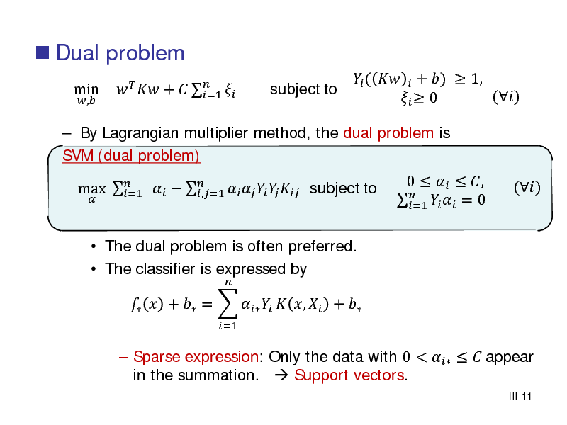
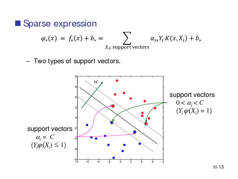
KKT condition
Theorem The solution of the primal and dual problem of SVM is given by the following equations: (1) (2) (3) (4) (6) (7) 1 + 0 ( ) 0 ( ) 0 , ( ) (1 ( + ) ) = 0 ( ) = 0 ( ), = 0, =1
[primal constraint] [primal constraint] [dual constraint] [complementary] [complementary]

(8) = 0, =1

III-12

Sparse expression

Two types of support vectors.
8

() = + =

: support vectors

, +

w
6 4

2

0

support vectors -2 i = C -4 (Yi(Xi) 1) -6

support vectors 0 < i < C (Yi (Xi) = 1)

-8 -8

-6

-4

-2

0

2

4

6

8

III-13

Summary of SVM
One of the kernel methods: kernelization of linear large margin classifier. Computation depends on Gram matrices of size .

Quadratic program: No local optimum. Many solvers are available. Further efficient optimization methods are available (e.g. SMO, Plat 1999) Sparse representation The solution is written by a small number of support vectors. Regularization The objective function can be regarded as regularization with hinge loss function.

III-14

NOT discussed on SVM in this lecture are Many successful applications Multi-class extension Combination of binary classifiers (1-vs-1, 1-vs-rest) Generalization of large margin criterion
Crammer & Singer (2001), Mangasarian & Musicant (2001), Lee, Lin, & Wahba (2004), etc

Other extensions Support vector regression (Vapnik 1995) -SVM (Schlkopf et al 2000) Structured-output (Collins & Duffty 2001, Taskar et al 2004, Altun
et al 2003, etc)

One-class SVM (Schkopf et al 2001) Optimization Solving primal problem Implementation (Chih-Jen Lins lecture)
III-15

References
Altun, Y., I. Tsochantaridis, and T. Hofmann. Hidden Markov support vector machines. In Proc. 20th Intern. Conf. Machine Learning, 2003. Boser, B.E., I.M. Guyon, and V.N. Vapnik. A training algorithm for optimal margin classifiers. In D. Haussler, editor, Fifth Annual ACM Workshop on Computational Learning Theory, pages 144152, Pittsburgh, PA, 1992. ACM Press. Crammer, K. and Y. Singer. On the algorithmic implementation of multiclass kernelbased vector machines. Journal of Machine Learning Research, 2:265292, 2001. Collins, M. and N. Duffy. Convolution kernels for natural language. In Advances in Neural Information Processing Systems 14, pages 625632. MIT Press, 2001. Mangasarian, O. L. and David R. Musicant. Lagrangian support vector machines. Journal of Machine Learning Research, 1:161177, 2001 Lee, Y., Y. Lin, and G. Wahba. Multicategory support vector machines, theory, and application to the classification of microarray data and satellite radiance data. Journal of the American Statistical Association, 99: 6781, 2004. Schlkopf, B., A. Smola, R.C. Williamson, and P.L. Bartlett. (2000) New support vector algorithms. Neural Computation, 12(5):12071245.
III-16

Schlkopf, B., J.C. Platt, J. Shawe-Taylor, R.C. Williamson, and A.J.Smola. (2001) Estimating the support of a high-dimensional distribution. Neural Computation, 13(7):14431471. Vapnik, V.N. The Nature of Statistical Learning Theory. Springer 1995. Platt, J. Fast training of support vector machines using sequential minimal optimization. In B. Schlkopf, C. Burges, and A. Smola, editors, Advances in Kernel Methods Support Vector Learning, pages 185208. MIT Press, 1999.

Books on Application domains: Lee, S.-W., A. Verri (Eds.) Pattern Recognition with Support Vector Machines: First International Workshop, SVM 2002, Niagara Falls, Canada, August 10, 2002. Proceedings. Lecture Notes in Computer Science 2388, Springer, 2002. Joachims, T. Learning to Classify Text Using Support Vector Machines: Methods, Theory and Algorithms. Springer, 2002. Schlkopf, B., K. Tsuda, J.-P. Vert (Eds.). Kernel Methods in Computational Biology. MIT Press, 2004.
III-17

IV. Theoretical Backgrounds of Kernel Methods
Kenji Fukumizu
The Institute of Statistical Mathematics / Graduate University for Advanced Studies September 6-7 Machine Learning Summer School 2012, Kyoto
1

-valued Positive definite kernel
Definition. : set. k : C is a positive definite kernel if for arbitrary 1, , and 1 , , ,

n

i , j =1 i

c c j k ( xi , x j ) 0.

Remark: From the above condition, the Gram matrix , necessarily Hermitian, i.e. , = (, ). [Exercise]

is

IV-2

Operations that preserve positive definiteness
Proposition 4.1 If : ( = 1,2, ,) are positive definite kernels, then so are the following: 1. (positive combination) 1 + 2 (, 0). 2. (product) 1 2 1 , 2 , 3. (limit) lim (, ), assuming the limit exists. Proof. 1 and 3 are trivial from the definition. For 2, it suffices to prove that Hadamard product (element-wise) of two positive semidefinite matrices is positive semidefinite.

Remark: The set of positive definite kernels on is a closed cone, where the topology is defined by the point-wise convergence.
IV-3

Proposition 4.2 Let and be positive semidefinite Hermitian matrices. Then, Hadamard product = (element-wise product) is positive semidefinite. Proof) Eigendecomposition of : = = i.e.,
Aij = p =1 pU ip U pj
n

p 0 by the positive semidefiniteness.

1 0 0 0 2 0 0

Then,

i , j=1 ci c j Kij = p=1 i , j=1 ci c j pU ipU pj Bij
n n n

= 1 i , j =1 ciU1i c jU1j Bij + + n
n

(

)

(

i ciU n c jU nj Bij 0. i , j =1

n

)

IV-4

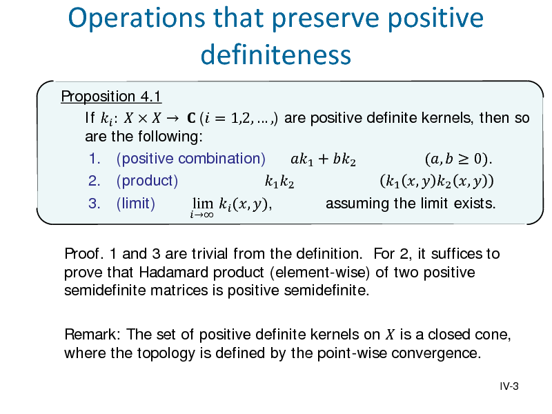
Normalization
Proposition 4.3 Let be a positive definite kernel on , and : be an arbitrary function. Then, is positive definite. In particular, , : = , () ()

is a positive definite kernel. Proof [Exercise] Example. Normalization: , =

is positive definite, and () = 1 for any .

(, )(, )

,

IV-5

Euclidean inner product : easy (Prop. 1.1). Gaussian RBF kernel exp Note exp 2
/2 2 2 2

Proof of positive definiteness

Polynomial kernel + ( 0): + = + 1 1 + + , 0. Product and non-negative combination of p.d. kernels. =
2 /2 /2

:

1 1 + =1+ 2 + 1! 2 2! 4 is positive definite (Prop. 4.1). Proposition 4.3 then completes the proof.
IV-6

2 /2

Laplacian kernel is discussed later.

A positive definite kernel , on is called shift-invariant if the kernel is of the form , = . Examples: Gaussian, Laplacian kernel , = exp 1 Fourier kernel (C-valued positive definite kernel): for each , = exp 1 exp (Prop. 4.3) 1

Shift-invariant kernel

If , = is positive definite, the function is called positive definite.

IV-7

Bochners theorem
Theorem 4.4 (Bochner) Let be a continuous function on . Then, is (-valued) positive definite if and only if there is a finite non-negative Borel measure on such that Bochners theorem characterizes all the continuous shift-invariant positive definite kernels. exp 1 is the generator of the cone (see Prop. 4.1). Sufficiency is easy: , = | Necessity is difficult.
1 |2

= exp

1 ()

is the inverse Fourier (or Fourier-Stieltjes) transform of . Roughly speaking, the shift invariant functions are the class that have non-negative Fourier transform.

IV-8

.

Suppose (shift-invariant) kernel has a form Then, RKHS is given by = , = exp 2 , 1
2

RKHS in frequency domain
. > 0.

where is the Fourier transform of : () =
1 ()exp 2

, =

< ,

1 .

IV-9

Gaussian kernel

, = exp 2 2

Laplacian kernel (on )
, = exp | | ,

1 , = 2 2 2 = 2 , exp 2 2 exp , = 2 2
2

2

2 exp 2
2

Decay of for high-frequency is different for Gaussian and IV-10 Laplacian.

= 2 ,

, = 2 2 +

=
2

2 + <

1 2 2 +

<

2

Polynomial kernel on : , = + ,
, 0 = 0 +

RKHS by polynomial kernel
2 2 1 1 + + . 0 1 + 0 1 2 0,

Span of these functions are polynomials of degree .

Proposition 4.5 If 0, the RKHS is the space of polynomials of degree at most . [Proof: exercise. Hint. Find to satisfy , = =0 =0 as a solution to a linear equation.]

IV-11

Sum

1 , 1 , 2 , 2 : two RKHSs and positive definite kernels on . RKHS for 1 + 2 : 1 + 2 = : 1 1 , 2 2 , = 1 + 2 }
2

Sum and product

Product

RKHS for 1 2 : 1 2 =tensor product as a vector space. =1
1

=

1

2 1

+ 2

2 2

= 1 + 2 , 1 1 , 2 2 }

= 1 , 2 } is dense in 1 2 . =1 , =1
1 2 2

= =1 =1

1

,

2

1

,
1

2

IV-12

2 .

Summary of Section IV
Positive definiteness of kernels are preserved by Non-negative combinations, Product Point-wise limit Normalization Bochners theorem: characterization of the continuous shiftinvariance kernels on .

Explicit form of RKHS RKHS with shift-invariance kernels has explicit expression in frequency domain. Polynomial kerns gives RKHS of polynomials. Sum and product can be given.
IV-13

References
Aronszajn., N. Theory of reproducing kernels. Trans. American Mathematical Society, 68(3):337404, 1950. Saitoh., S. Integral transforms, reproducing kernels, and their applications. Addison Wesley Longman, 1997.

IV-14

Solution to Exercises
C-valued positive definiteness
Using the definition for one point, we have , is real and nonnegative for all . For any and , applying the definition with coefficient (, 1) where , we have 2 , + , + , + , 0. Since the right hand side is real, its complex conjugate also satisfies 2 , + , + , + , 0. The difference of the left hand side of the above two inequalities is real, so that , , ( , , ) holds for any . This implies , = (, ).

is a real number. On the other hand, since must be pure imaginary for any complex number , , , = 0

IV-15

V. Nonparametric Inference with Positive Definite Kernels
Kenji Fukumizu
The Institute of Statistical Mathematics / Graduate University for Advanced Studies September 6-7 Machine Learning Summer School 2012, Kyoto
1

Outline
1. Mean and Variance on RKHS 2. Statistical tests with kernels 3. Conditional probabilities and beyond.

V-2

Introduction
Kernel methods for statistical inference
We have seen that kernelization of linear methods provides nonlinear methods, which capture nonlinearity or high-order moments of original data. e.g. nonlinear SVM, kernel PCA, kernel CCA, etc. This section discusses more basic statistics on RKHS (X) = k( , X) X (original space) feature map

H (RKHS) mean, covariance, conditional covariance
V-3

MeanandcovarianceonRKHS

V-4

MeanonRKHS
X: random variable taking value on a measurable space k: measurable positive definite kernel on . H: RKHS. Always assumes bounded kernel for simplicity: sup , .

( X ) k ( , X ) : feature vector = random variable on RKHS.
Definition. The kernel mean of X on H is defined by

Reproducing expectation:

,
m X , f E f ( X )

.

* Notation:

depends on , also. But, we do not show it for simplicity.
V-5 5

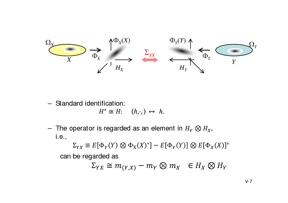
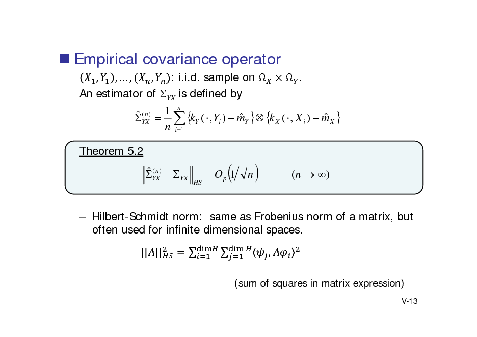
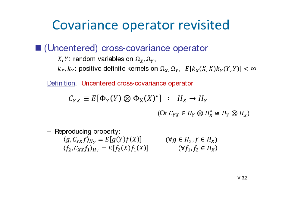
Covarianceoperator
, : random variable taking values on , , resp. , , , : RKHS given by kernels on and , resp. Definition. Cross-covariance operator: YX : H X H Y

, :

,

denotes the linear functional

Simply, covariance of feature vectors. c.f. Euclidean case VYX = E[YXT] E[Y]E[X]T : covariance matrix Reproducing covariance:

g , YX f E[ g (Y ) f ( X )] E[ g (Y )]E[ f ( X )] ( Cov[ f ( X ), g (Y )])
for all , .
V-6

X X X

X(X)

Y(Y)

YX
HX HY

Y Y Y

Standard identification: :

,, . ,

The operator is regarded as an element in i.e., can be regarded as

,

V-7

Characteristickernel
(Fukumizu,Bach,Jordan2004,2009;Sriperumbudur etal2010)

Kernel mean can capture higher-order moments of the variable. Example X: R-valued random variablek: pos.def. kernel on R. Suppose k admits a Taylor series expansion on R.

k (u , x) c0 c1 ( xu ) c2 ( xu ) 2

(ci > 0)
e.g.) k ( x, u ) exp( xu )

The kernel mean mX works as a moment generating function:

m X (u ) E[k (u , X )] c0 c1 E[ X ]u c2 E[ X 2 ]u 2
1 d m X (u ) E[ X ] c du u 0
V-8

P : family of all the probabilities on a measurable space (, B).
H: RKHS on with a bounded measurable kernel k. mP: kernel mean on H for a variable with probability P P
Definition. A bounded measureable positive definite k is called characteristic (w.r.t. P) if the mapping

P H,
is one-to-one.

P mP

The kernel mean with a characteristic kernel uniquely determines a probability.

mP mQ
i.e.
~

PQ
.
V-9

Analogy to characteristic function With Fourier kernel F ( x, y ) exp 1 x T y

Ch.f. X (u) E[ F ( X , u)].
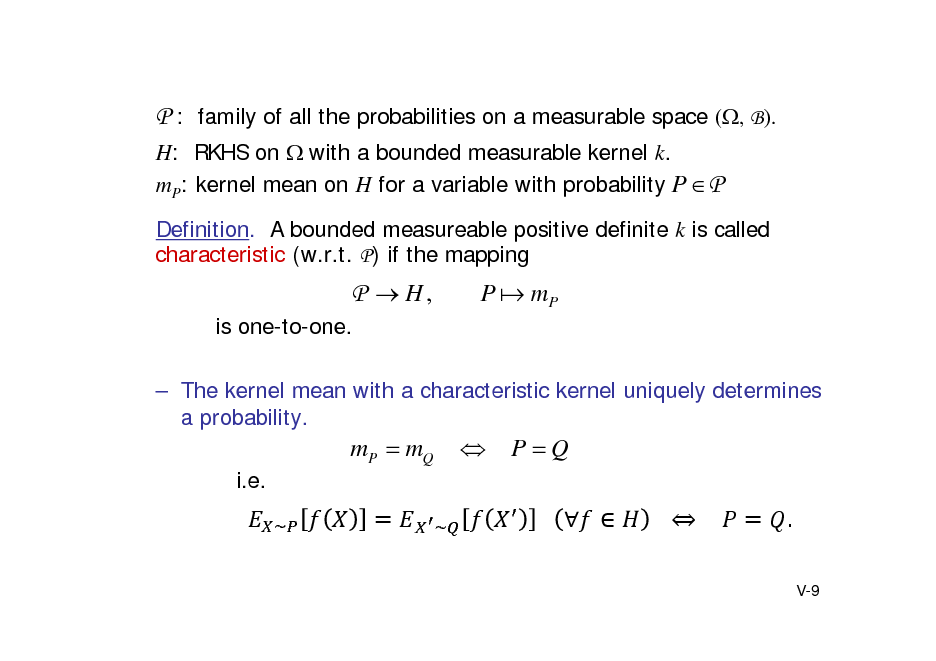
The characteristic function uniquely determines a Borel probability on Rm. The kernel mean m X (u ) E[ k (u , X )] with a characteristic kernel uniquely determines a probability on (, B). Note: may not be Euclidean.

The characteristic RKHS must be large enough! Examples for Rm (proved later): Gaussian, Laplacian kernel. Polynomial kernels are not characteristic.

V-10

Statisticalinferencewithkernelmeans
Statistical inference: inference on some properties of probabilities. With characteristic kernels, they can be cast into the inference on kernel means. Two sample problem: Independence test: ? ? ? ?

V-11

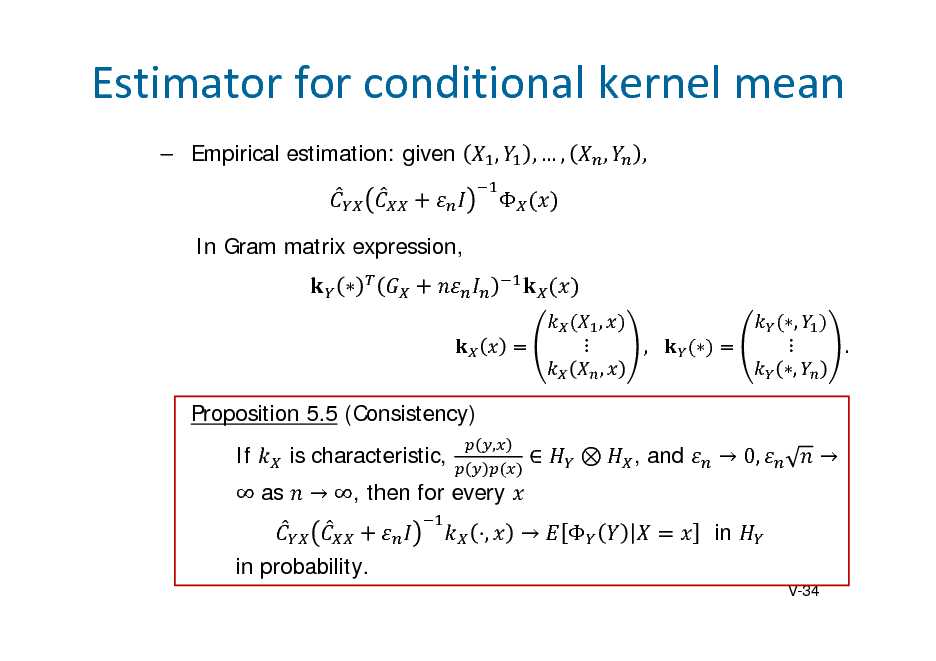
EmpiricalEstimation
Empirical kernel mean
An advantage of RKHS approach is easy empirical estimation.

X 1 ,..., X n : i.i.d.

X 1 ,, X n

: sample on RKHS

Empirical mean:

m(Xn )

1 n 1 n ( X i ) k ( , X i ) n i 1 n i 1

-consistency) Theorem 5.1 (strong Assume E[ k ( X , X )] .

m (Xn ) m X O p 1

n

( n ).

V-12

Empirical covariance operator
, ,, , : i.i.d. sample on . An estimator of YX is defined by 1 n (n) YX kY ( , Yi ) mY k X ( , X i ) m X n i 1 Theorem 5.2

(n YX) YX

HS

Op 1

n

(n )

Hilbert-Schmidt norm: same as Frobenius norm of a matrix, but often used for infinite dimensional spaces. | | ,
(sum of squares in matrix expression)
V-13

Statisticaltestwithkernels

V-14

Twosampleproblem
Two sample homogeneity test Two i.i.d. samples are given;

X 1 ,..., X n ~ P

and

Y1 ,..., Y ~ Q.

Q: Are they sampled from the same distribution? Null hypothesis H0: . Alternative H1: . Practically important: we often wish to distinguish two things.
Are the experimental results of treatment and control significantly different? Were the plays Henry VI and Henry II written by the same author?

If then means of and are different, we may use it for test. If they are identical, we need to look at higher order information.
V-15

If mean and variance are the same, it is a very difficult problem. Example: do they have the same distribution? 100
4 4 4 3 3 3

2

2

2

1

1

1

0

0

0

-1

-1

-1

-2

-2

-2

-3

-3

-3

-4 -4

-3

-2

-1

0

1

2

3

4

-4 -4

-3

-2

-1

0

1

2

3

4

-4 -4

-3

-2

-1

0

1

2

3

4

4

4

4

3

3

3

2

2

2

1

1

1

0

0

0

-1

-1

-1

-2

-2

-2

-3

-3

-3

-4 -4

-3

-2

-1

0

1

2

3

4

-4 -4

-3

-2

-1

0

1

2

3

4

-4 -4

-3

-2

-1

0

1

2

3

4

V-16

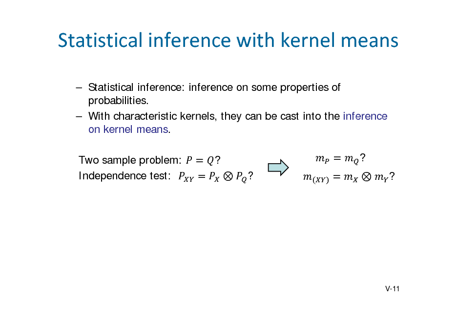
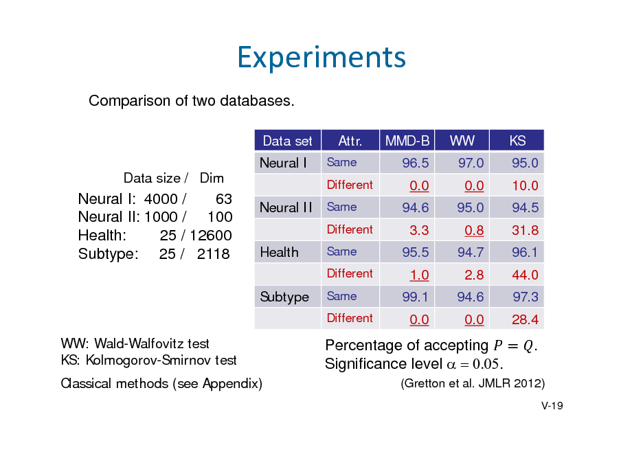
Kernel method for two-sample problem
(Gretton et al. NIPS 2007, 2010, JMLR2012).

Kernel approach
Comparison of and comparison of and .

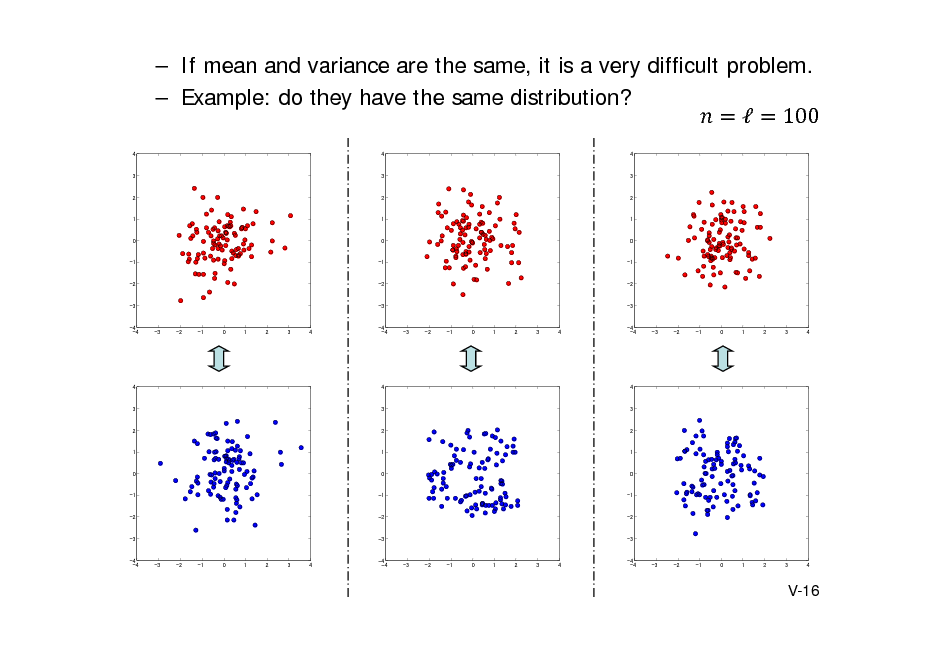
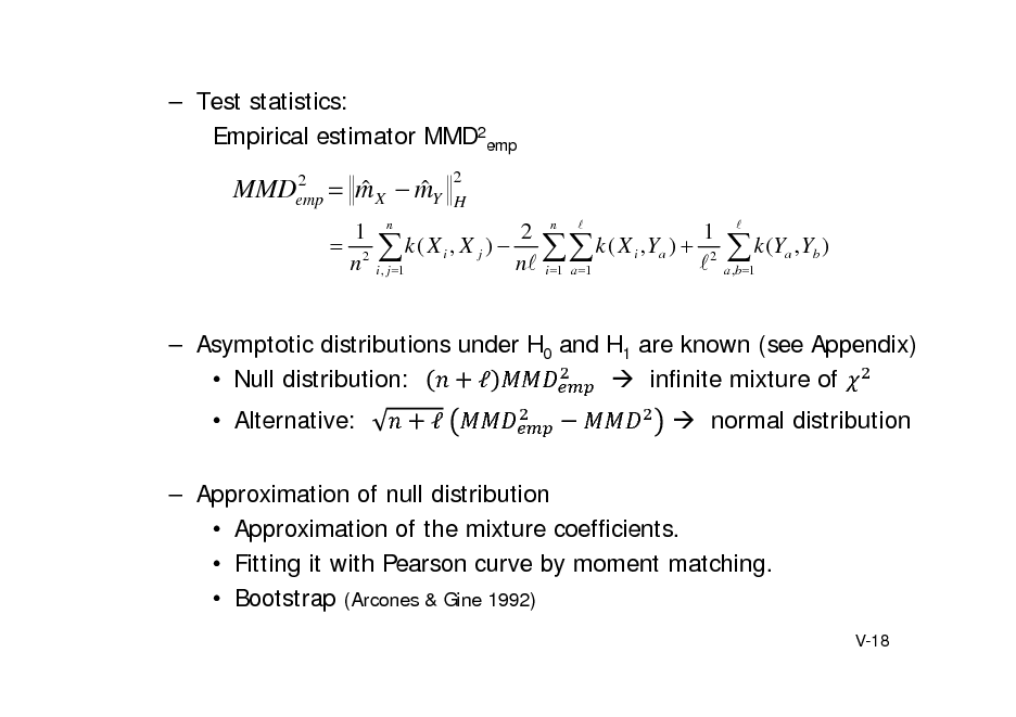
Maximum Mean Discrepancy
In population

MMD 2 m X mY

2 H

~ ~ E[k ( X , X )] E[k (Y , Y )] 2 E[k ( X , Y )].
( , : independent copy of , )

m X mY

H

sup

f :|| f ||H 1

f , m X mY sup

f :|| f ||H 1

f ( x )dP( x ) f ( x )dQ ( x )
hence, MMD.

With characteristic kernel, MMD = 0 if and only if

.
V-17

Test statistics: Empirical estimator MMD2emp
2 MMDemp

m X mY

2 H

1 n 2 n 1 2 k ( X i , X j ) k ( X i , Ya ) 2 n i , j 1 n i 1 a 1

a ,b 1

k (Y ,Y )
a b

Asymptotic distributions under H0 and H1 are known (see Appendix) Null distribution: infinite mixture of Alternative: normal distribution

Approximation of null distribution Approximation of the mixture coefficients. Fitting it with Pearson curve by moment matching. Bootstrap (Arcones & Gine 1992)
V-18

Experiments
Comparison of two databases.
Data set Neural I Data size / Dim Attr.
Same Different

MMD-B 96.5 0.0 94.6 3.3 95.5 1.0 99.1 0.0

WW 97.0 0.0 95.0 0.8 94.7 2.8 94.6 0.0

KS 95.0 10.0 94.5 31.8 96.1 44.0 97.3 28.4

Neural I: 4000 / 63 Neural II: 1000 / 100 Health: 25 / 12600 Subtype: 25 / 2118

Neural II Same
Different

Health Subtype

Same Different Same Different

WW: Wald-Walfovitz test KS: Kolmogorov-Smirnov test Classical methods (see Appendix)

Percentage of accepting Significance level .

.

(Gretton et al. JMLR 2012)
V-19

Experimentsformixtures
0.03 0.025 0.02 0.015 0.01 0.005 0.005 0 0 0.2 0.4 0.6 0.8 1 0 0 0.2 0.4 0.6 0.8 1 0.01

NX = NY = 100

0.02

NX = NY = 200

0.015

c

0.014

Average values of MMD over 100 samples 0,1 vs Unif 1 0,1 vs 0,1 0,1

0.012 0.01 0.008 0.006 0.004 0.002 0

NX = NY = 500

0

0.2

0.4

0.6

0.8

1

20

Independencetest
Independence
and are independent if and only if Probability density function: Cumulative distribution function: Characteristic function: , , . .

Independence test
Given i.i.d. sample , Null hypothesis H0: Alternative H1: ,, , , are and independent? (independent) (not independent)

V-21

Independent
3 3 2 2

Dependent

1

1

0

0

-1

-1

-2

-2

-3 -3

-2

-1

0

1

2

3

-3 -3

-2

-1

0

1

2

3

V-22

Independencewithkernel
Theorem 5.3. (Fukumizu, Bach, Jordan, JMLR 2004) If the product kernel is characteristic, then

X Y YX O
Recall . Comparison between (kernel mean of (kernel mean of ). ) and

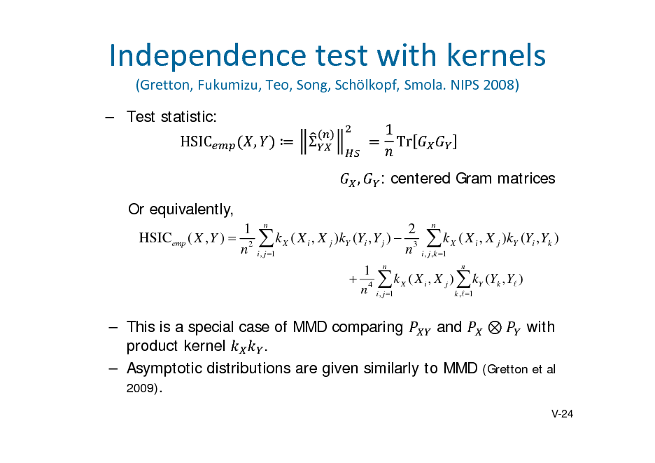
Dependence measure: Hilbert-Schmidt independence criterion , , 2
, : independent copy of ,

[Exercise]

, ,
.

, ,

,

V-23

Independencetestwithkernels
(Gretton,Fukumizu,Teo,Song,Schlkopf,Smola.NIPS2008) Test statistic: HSIC , , Or equivalently,
1 n 2 n HSICemp ( X , Y ) 2 k X ( X i , X j )kY (Yi , Y j ) 3 k X ( X i , X j )kY (Yi , Yk ) n i , j 1 n i , j ,k 1 n 1 n 4 k X ( X i , X j ) kY (Yk , Y ) n i , j 1 k , 1

1

Tr

: centered Gram matrices

and with This is a special case of MMD comparing product kernel . Asymptotic distributions are given similarly to MMD (Gretton et al 2009).
V-24

Comparisonwithexistingmethod
Distance covariance
(Szkely et al., 2007; Szkely & Rizzo, 2009)

Distance covariance / distance correlation has gained popularity in statistical community as a dependence measure beyond Pearson correlation. Definition. , : and -dimensional random vectors .

Distance covariance: , 2
where ,

and , are i.i.d. ~

|
.

Distance correlation: , , , ,
V-25

Relation between distance covariance and MMD
Proposition 5.4 (Sejdinovic, Gretton, Sriperumbudur, F. ICML2012) A kernel on Euclidean spaces , . is positive definite, and , , . HSIC Distance covariance is a specific instance of MMD. Positive definite kernel approach is more general in choosing kernels, and thus may perform better. Extension , is positive definite for 0 , HSIC 2. We can define ,
V-26

Experiments
Ratio of accepting independence

Original distance covariance

2

HSIC with Gaussian kernel

Dependence
V-27

Choice of kernel for MMD
Heuristics for Gaussian kernel: median , 1, ,

Using performance of statistical test: Type II error of the test statistics (Gretton et al NIPS 2012). Challenging open questions.

V-28

Conditionalprobabilitiesand beyond

V-29

Conditionalprobability
Conditional probabilities appear in many machine learning problems Regression / classification: direct inference of | or | . already seen in Section II. Bayesian inference Conditional independence / dependence Graphical modeling X1 Conditional independent relations among variables. Causality Dimension reduction / feature extraction

X2

X3

X4

X5

V-30

Conditionalkernelmean
Conditional kernel mean
Definition. ,

Simply, kernel mean of | . It determines the conditional probability with a characteristic kernel. Again, inference problems on conditional probabilities can be solved as inference on conditional kernel means. But, how can we estimate it?

V-31

Covarianceoperatorrevisited
(Uncentered) cross-covariance operator
, : random variables on , , , : positive definite kernels on , , Definition. Uncentered cross-covariance operator , , .

(Or Reproducing property: , ,

)

, ,

V-32

Conditionalprobabilitybyregression
Recall for zero-mean Gaussian random variable . Given by the solution to the least mean square , For the feature vector . , ,

Given by the solution to the least mean square , is not well defined in infinite dimensional cases, but regularized estimator can be justified.
V-33

Estimatorforconditionalkernelmean
Empirical estimation: given , In Gram matrix expression,
, , , , , .

,,

,

,

Proposition 5.5 (Consistency) If as is characteristic, , in probability.
V-34

,

, and

0, in

, then for every

Conditionalcovariance
Review: Gaussian variables
Conditional covariance matrix: Fact:
| |

for any

Cov , |

Conditional cross-covariance operator
Definition: , , : random variables on , , . , , : positive definite kernel on , , . Conditional cross-covariance operator
|

, ,

Reproducing averaged conditional covariance Proposition 5.6 If is characteristic, then for ,
|

Cov

,

|

V-35

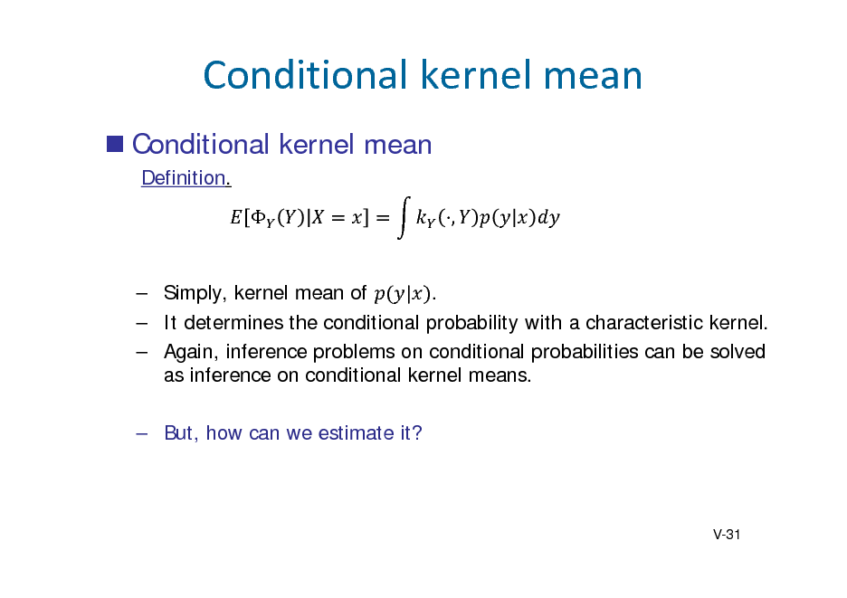
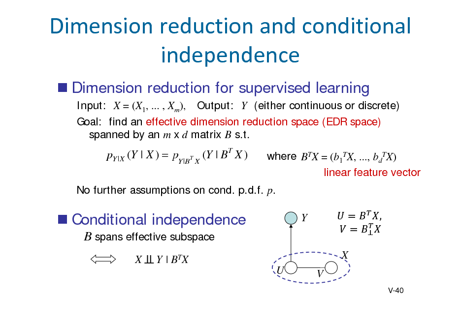
An interpretation: Compare the conditional kernel means for , and | . |

Dependence on

is not easy to handle Average it out. | ]

Empirical estimator: |

V-36

Conditionalindependence
Recall: for Gaussian random variable | . | does not imply conditional By average over , | independence, which requires , | for each . Trick: consider
|

,

, and the product kernel is used for .

where

Theorem 5.7 (Fukumizu et al. JMLR 2004) Assume , , are characteristic, then | . |
|

,

|

can be similarly used.

V-37

Applicationsofconditional dependencemeasures
Conditional independence test
Squared HS-norm independence test. Unlike the independence test, the asymptotic null distribution is not available. Permutation test is needed. Background: The conditional independent test with continuous non-Gaussian variables is not easy, and a challenging open problem.
|

(Fukumizu et al. NIPS2007)

can be used for conditional

V-38

Causal inference
Directional acyclic graph (DAG) is used for representing the causal structure among variables. The structure can be learned by conditional independence tests. The above test can be applied (Sun, Janzing, Schlkopf, F. ICML2007).

X

Y
and

X X

Y Y |Z

Z

Feature extraction / dimension reduction for supervised learning see next.

V-39

Dimensionreductionandconditional independence
Dimension reduction for supervised learning
Input: X = (X1, ... , Xm), Output: Y (either continuous or discrete) Goal: find an effective dimension reduction space (EDR space) spanned by an m x d matrix B s.t.

pY | X (Y | X ) pY |BT X (Y | BT X )

where BTX = (b1TX, ..., bdTX) linear feature vector

No further assumptions on cond. p.d.f. p.

Conditional independence
B spans effective subspace
X Y | BTX U

Y X V

,

V-40

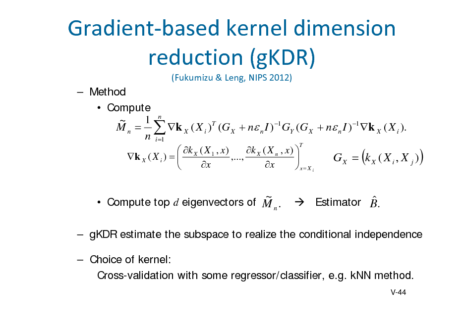
Gradientbasedmethod
(Samarov 1993;Hristache etal2001)

Average Derivative Estimation (ADE)
Assumptions: Y is one dimensional EDR space p (Y | X ) ~ (Y | B T X ) p

~ ( y | B T x)dy B y ~ ( y | z ) T dy E[Y | X x] yp z p zB x x x
Gradient of the regression function lies in the EDR space at each x

B = average or PCA of the gradients at many x.

V-41

KernelHelps!
Weakness of ADE: Difficulty of estimating gradients in high dimensional space. ADE uses local polynomial regression. Sensitive to bandwidth May find only a subspace of the effective subspace. e.g.

Y ~ f ( X1) Z ,

Z ~ N (0, ( X 2 ) 2 ).

Kernel method Can handle conditional probability in regression form Characterizes conditional independence X

Y | BTX

V-42

Derivativewithkernel
Reproducing the derivative (e.g. Steinwart & Christmann, Chap. 4):

k X ( , x ) k X ( x, ~ ) is differentiable and x Assume H X then x

k X ( , x ) f ( x ) f, x x

for any

Combining with the estimation of conditional kernel mean, ij ( x ) E [ Y (Y ) | X x ] , E [ Y (Y ) | X x ] M x i x j

k ( , x ) k ( , x ) CYX (C XX n I ) 1 X , CYX (C XX n I ) 1 X xi x j
The top eigenvectors of estimates the EDR space
V-43

Gradientbasedkerneldimension reduction(gKDR)
(Fukumizu&Leng,NIPS2012)

Method Compute 1 n ~ M n k X ( X i )T (G X n n I ) 1 GY (G X n n I ) 1 k X ( X i ). n i 1
k ( X , x ) k ( X , x ) k X ( X i ) X 1 ,..., X n x x x X i
T

G X k X ( X i , X j )

Compute top d eigenvectors of M n .

~

Estimator B.

gKDR estimate the subspace to realize the conditional independence Choice of kernel: Cross-validation with some regressor/classifier, e.g. kNN method.
V-44

Experiment:ISOLET
Speech signals of 26 alphabets 617 dim. (continuous) 6238 training data / 1559 test data Results
Dim Dim 10 15 7.50 7.57 8.66 20 5.00 4.75 6.54 25 4.75 4.30 6.09 30 3.85 35 3.85 40 3.59 45 3.53 50 3.08 gKDR 14.43 gKDR gKDR-v gKDR-v 16.87 CCA CCA 13.09

Data from UCI repository.

Classification errors for test data by SVM (%) c.f. C4.5 + ECOC: 6.61% Neural Networks (best): 3.27%
V-45

Experiment:AmazonCommerceReviews
Author identification for Amazon commerce reviews. Dim = 10000 (linguistic style: e.g. usage of digit, punctuation, words and sentences' length, and frequency of words, etc) = #authors x 30 (Data from UCI repository.)

V-46

Example of 2-dim plots for 3 authors

gKDR (dim = #authors) vs correlation-based variable selection (dim=500/2000)
#Authors gKDR + 5NN 9.3 16.2 20.1 22.8 22.7 gKDR + SVM 12.0 16.2 18.0 21.8 19.5 Corr (500) + SVM 15.7 30.2 29.2 35.4 41.1 Corr (2000) + SVM 8.3 18.0 24.0 25.0 29.0
V-47

10 20 30 40 50

10-fold cross-validation errors (%)

Bayesianinferencewithkernels
(Fukumizu,Song,GrettonNIPS2011)

Bayes rule
, .

Kernel Bayes rule
| : kernel mean of prior, , : kernel representation of relation between and , , ,, , ~ , i.i.d. | .

Goal: compute kernel mean of posterior
|

| |

,

Diag

V-48

Bayesianinferenceusingkernel Bayes'rule
NO PARAMETRIC MODELS, BUT SAMPLES! When is it useful? is Explicit form of cond. p.d.f. | or prior unavailable, but sampling is easy. Approximate Bayesian Computation (ABC), Process prior. Cond. p.d.f. | is unknown, but sample from , is given in training phase. Example: nonparametric HMM (shown later). If both of | and are known, there are many good sampling methods, such as MCMC, SMC, etc. But, they may take long time. KBR uses matrix operations.

V-49

Application:nonparametricHMM
Model: , | Assume: XT X0 X1 X2 X3 | and/or | is not known. But, data , is available Y0 Y1 Y2 Y3 YT in training phase. Examples: Measurement of hidden states is expensive, Hidden states are measured with time delay. Testing phase (e.g., filtering, e.g.): given , , , estimate hidden state .

Sequential filtering/prediction uses Bayes rule KBR applied.

V-50

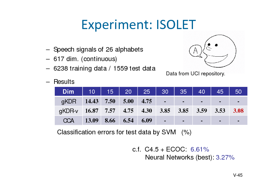
Camera angles
Hidden : angles of a video camera located at a corner of a room. Observed : movie frame of a room + additive Gaussian noise. : 3600 downsampled frames of 20 x 20 RGB pixels (1200 dim. ). The first 1800 frames for training, and the second half for testing

noise

KBR (Trace) 0.15 0.01

Kalman filter(Q) 0.56 0.54 0.02 0.02

2 = 10-4 2 = 10-3

0.21 0.01

Average MSE for camera angles (10 runs) To represent SO(3) model, Tr[AB-1] for KBR, and quaternion expression for Kalman filter are used .
V-51

SummaryofPartV
Kernel mean embedding of probabilities
Kernel mean gives a representation of probability distribution. Inference on probabilities can be cast into inference on kernel means. e.g. two sample test, independent test

Conditional probabilities
Conditional probabilities can be handled with kernel means and covariances Conditional independence test Graphical modeling Causal inference Dimension reduction Bayesian inference
V-52

References
Fukumizu, K., Bach, F.R., and Jordan, M.I. (2004) Dimensionality reduction for supervised learning with reproducing kernel Hilbert spaces. Journal of Machine Learning Research. 5:73-99, Fukumizu, K., F.R. Bach and M. Jordan. (2009) Kernel dimension reduction in regression. Annals of Statistics. 37(4), pp.1871-1905 Fukumizu, K., L. Song, A. Gretton (2011) Kernel Bayes' Rule. Advances in Neural Information Processing Systems 24 (NIPS2011) 1737-1745. Gretton, A., K.M. Borgwardt, M.Rasch, B. Schlkopf, A.J. Smola (2007) A Kernel Method for the Two-Sample-Problem. Advances in Neural Information Processing Systems 19, 513-520. Gretton, A., Z. Harchaoui, K. Fukumizu, B. Sriperumbudur (2010) A Fast, Consistent Kernel Two-Sample Test. Advances in Neural Information Processing Systems 22, 673-681. Gretton, A., K. Fukumizu, C.-H. Teo, L. Song, B. Schlkopf, A. Smola. (2008) A Kernel Statistical Test of Independence. Advances in Neural Information Processing Systems 20, 585-592. Gretton, A., K. Fukumizu, C.-H. Teo, L. Song, B. Schlkopf, A. Smola. (2008) A Kernel Statistical Test of Independence. Advances in Neural Information Processing Systems 20, 585-592. V-53

Hristache, M., A. Juditsky, J. Polzehl, and V. Spokoiny. (2001) Structure Adaptive Approach for Dimension Reduction. Annals of Statsitics, 29(6):1537-1566. Samarov, A. (1993). Exploring regression structure using nonparametric functional estimation. Journal of American Statistical Association. 88, 836-847. Sejdinovic, D., A. Gretton, B. Sriperumbudur, K. Fukumizu. (2012) Hypothesis testing using pairwise distances and associated kernels. Proc. 29th International Conference on Machine Learning (ICML2012). Sriperumbudur, B.K., A. Gretton, K. Fukumizu, B. Schlkopf, G.R.G. Lanckriet. (2010) Hilbert Space Embeddings and Metrics on Probability Measures. Journal of Machine Learning Research. 11:1517-1561. Sun, X., D. Janzing, B. Schlkopf and K. Fukumizu. (2007) A kernel-based causal learning algorithm. Proc. 24th Annual International Conference on Machine Learning (ICML2007), 855-862. Szkely, G.J., M.L. Rizzo, and N.K. Bakirov. (2007) Measuring and testing dependence by correlation of distances. Annals of Statistics, 35(6): 2769-2794. Szkely, G.J. and M.L. Rizzo. (2009) Brownian distance covariance. Annals of Applied Statistics, 3(4):1236-1265.

V-54

Appendices

V-55

StatisticalTest:quickintroduction
How should we set the threshold?
Example) Based on MMD, we wish to make a decision whether the two variables have the same distribution. Simple-minded idea: Set a small value like t = 0.001 MMD(X,Y) < t Perhaps, same MMD(X,Y) t Different But, the threshold should depend on the properties of X and Y.

Statistical hypothesis test
A statistical way of deciding whether a hypothesis is true or not. The decision is based on sample We cannot be 100% certain.
V-56

Procedure of hypothesis test
Null hypothesis H0 = hypothesis assumed to be true X and Y have the same distribution Prepare a test statistic TN e.g.

TN = MMDemp2

Null distribution: Distribution of TN under H0 Set significance level Typically = 0.05 or 0.01 Compute the critical region: = Pr(TN > t under H0) Reject the null hypothesis if TN > t The probability that MMDemp2 > t under H0 is very small. otherwise, accept H0 negatively.
V-57

One-sided test
1 0.9 0.8 0.7 0.6 0.5 0.4 0.3 0.2 0.1 0

p.d.f. of Null distribution area = p-value

TN > t p-value <

area = (5%, 1% etc) significance level
0 0.5 1 1.5 2 2.5 3 3.5 4 4.5 5

TN
threshold t

critical region

- If H0 is the truth, the value of TN should follow the null distribution. - If H1 is the truth, the value of TN should be very large. - Set the threshold with risk . - The threshold depends on the distribution of the data.
V-58

Type I and Type II error
Type I error = false positive (e.g. = positive) Type II error = false negative TRUTH H0 Alternative Reject H0 Accept H0 TEST RESULT True negative Type II error False negative Type I error False positive

True positive

Significance level controls the type I error. Under a fixed type I error, a good test statistics should give small type II error.
V-59

MMD:Asymptoticdistribution
Under H0
, , ~ , , , ~ : i.i.d. Let (0 1) as Assume , 1 Under the null hypothesis of MMD

. .

, 1 1 , , and are

where , , are i.i.d. with law 0; 1/ 1 the eigenvalues of the integral operator on , with the centered kernel , , ,

,

,

.
V-60

: independent copy of .

Under H1

Under the alternative MMD where 4
, ,

, 0; ,

,

,

.

The asymptotic distributions are derived by the general theory of U-statistics (e.g. see van der Vaart 1998, Chapter 12). Estimation of the null distribution: Estimation of Approximation by Pearson curve with moment matching. Bootstrap MMD (Arcones & Gine 1992)
V-61

Kolmogorov-Smirnov (K-S) test for two samples
One-dimensional variables Empirical distribution function

Conventionalmethodsfortwo sampleproblem
1 N FN (t ) I ( X i t ) N i 1

KS test statistics

DN

1 sup FN (t ) tR

2 FN (t )

FN2(t) DN FN1(t)

Asymptotic null distribution is known (not shown here).

t

V-62

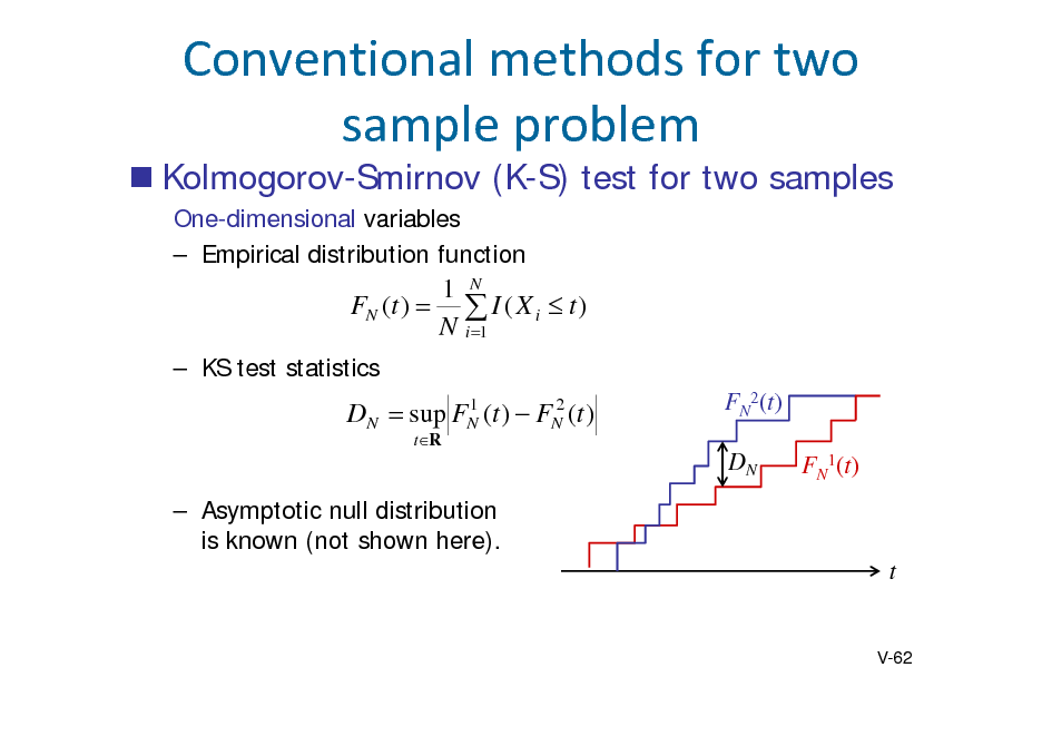
Wald-Wolfowitz run test
One-dimensional samples Combine the samples and plot the points in ascending order. Label the points based on the original two groups. Count the number of runs, i.e. consecutive sequences of the same label. Test statistics R = Number of runs

TN

R E[ R ] Var[ R ]

N (0,1)
R = 10

In one-dimensional case, less powerful than KS test

Multidimensional extension of KS and WW test
Minimum spanning tree is used (Friedman Rafsky 1979)
V-63