Statistical Learning Theory
Machine Learning Summer School, Kyoto, Japan

Alexander (Sasha) Rakhlin
University of Pennsylvania, The Wharton School Penn Research in Machine Learning (PRiML)

August 27-28, 2012

1 / 130

References

Parts of these lectures are based on O. Bousquet, S. Boucheron, G. Lugosi: Introduction to Statistical Learning Theory, 2004. MLSS notes by O. Bousquet S. Mendelson: A Few Notes on Statistical Learning Theory Lecture notes by S. Shalev-Shwartz Lecture notes (S. R. and K. Sridharan)
http://stat.wharton.upenn.edu/~rakhlin/courses/stat928/stat928_notes.pdf

Prerequisites: a basic familiarity with Probability is assumed.

2 / 130

Outline
Introduction Statistical Learning Theory The Setting of SLT Consistency, No Free Lunch Theorems, Bias-Variance Tradeo Tools from Probability, Empirical Processes From Finite to Innite Classes Uniform Convergence, Symmetrization, and Rademacher Complexity Large Margin Theory for Classication Properties of Rademacher Complexity Covering Numbers and Scale-Sensitive Dimensions Faster Rates Model Selection Sequential Prediction / Online Learning Motivation Supervised Learning Online Convex and Linear Optimization Online-to-Batch Conversion, SVM optimization

3 / 130

Example #1: Handwritten Digit Recognition
Imagine you are asked to write a computer program that recognizes postal codes on envelopes. You observe the huge amount of variation and ambiguity in the data:

One can try to hard-code all the possibilities, but likely to fail. It would be nice if a program looked at a large corpus of data and learned the distinctions!

4 / 130

This picture of MNIST dataset was yanked from http://www.heikohomann.de/htmlthesis/node144.html

Example #1: Handwritten Digit Recognition
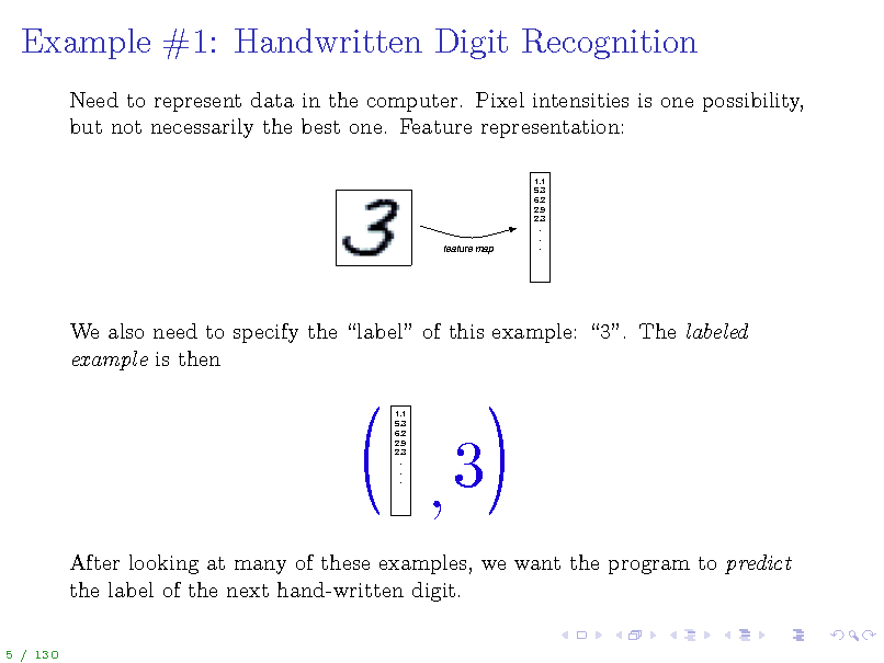
Need to represent data in the computer. Pixel intensities is one possibility, but not necessarily the best one. Feature representation:

feature map

We also need to specify the label of this example: 3. The labeled example is then
1.1 5.3 6.2 2.9 2.3 . . .

After looking at many of these examples, we want the program to predict the label of the next hand-written digit.
5 / 130

(

,3

(

1.1 5.3 6.2 2.9 2.3 . . .

Example #2: Predict Topic of a News Article
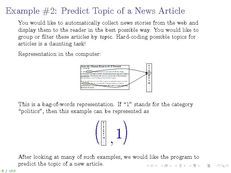
You would like to automatically collect news stories from the web and display them to the reader in the best possible way. You would like to group or lter these articles by topic. Hard-coding possible topics for articles is a daunting task! Representation in the computer:
0 1 0 2 5 0 1 10 . . .

This is a bag-of-words representation. If 1 stands for the category politics, then this example can be represented as
0 1 0 2 5 0 1 10 . . .

After looking at many of such examples, we would like the program to predict the topic of a new article.
6 / 130

(

,1

(

Why Machine Learning?

Impossible to hard-code all the knowledge into a computer program. The systems need to be adaptive to the changes in the environment. Examples: Computer vision: face detection, face recognition Audio: voice recognition, parsing Text: document topics, translation Ad placement on web pages Movie recommendations Email spam detection

7 / 130

Machine Learning

(Human) learning is the process of acquiring knowledge or skill. Quite vague. How can we build a mathematical theory for something so imprecise? Machine Learning is concerned with the design and analysis of algorithms that improve performance after observing data. That is, the acquired knowledge comes from data. We need to make mathematically precise the following terms: performance, improve, data.

8 / 130

Learning from Examples
How is it possible to conclude something general from specic examples? Learning is inherently an ill-posed problem, as there are many alternatives that could be consistent with the observed examples. Learning can be seen as the process of induction (as opposed to deduction): extrapolating from examples. Prior knowledge is how we make the problem well-posed. Memorization is not learning, not induction. Our theory should make this apparent. Very important to delineate assumptions. Then we will be able to prove mathematically that certain learning algorithms perform well.

9 / 130

Data
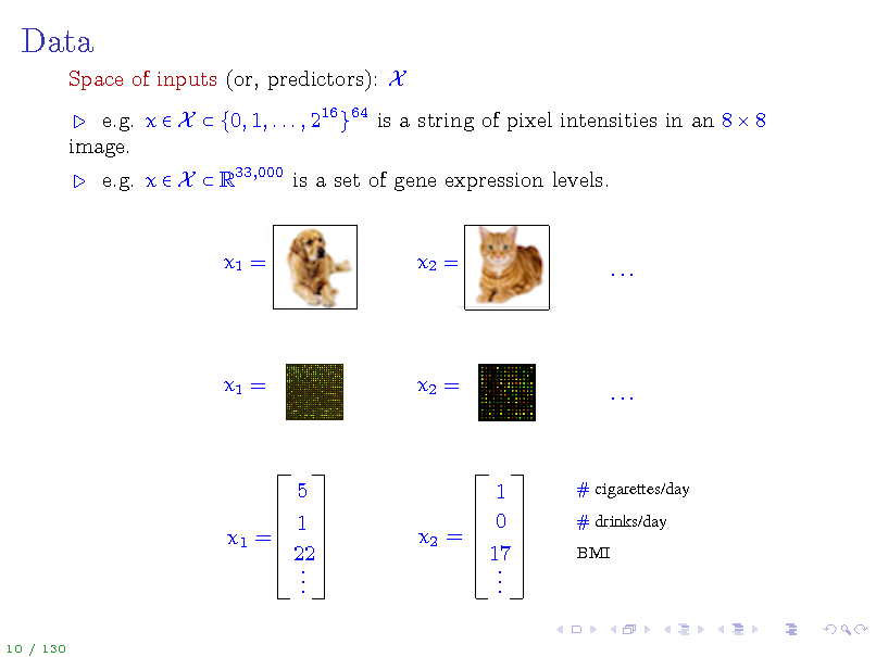
Space of inputs (or, predictors): X e.g. x X {0, 1, . . . , 216 }64 is a string of pixel intensities in an 8 8 image. e.g. x X R33,000 is a set of gene expression levels.

x1 =

x2 =

...

x1 =

x2 =

...

x1 =

5 1 22 ...

x2 =

1 0 17 ...

# cigarettes/day # drinks/day BMI

10 / 130

Data

Sometimes the space X is uniquely dened for the problem. In other cases, such as in vision/text/audio applications, many possibilities exist, and a good feature representation is key to obtaining good performance.

This important part of machine learning applications will not be discussed in this lecture, and we will assume that X has been chosen by the practitioner.

11 / 130

Data

Space of outputs (or, responses): Y e.g. y Y = {0, 1} is a binary label (1 = cat) e.g. y Y = [0, 200] is life expectancy A pair (x, y) is a labeled example. e.g. (x, y) is an example of an image with a label y = 1, which stands for the presence of a face in the image x Dataset (or training data): examples (x1 , y1 ), . . . , (xn , yn ) e.g. a collection of images labeled according to the presence or absence of a face

12 / 130

The Multitude of Learning Frameworks
Presence/absence of labeled data: Supervised Learning: (x1 , y1 ), . . . , (xn , yn ) Unsupervised Learning: x1 , . . . , xn Semi-supervised Learning: a mix of the above This distinction is important, as labels are often dicult or expensive to obtain (e.g. can collect a large corpus of emails, but which ones are spam?) Types of labels: Binary Classication / Pattern Recognition: Y = {0, 1} Multiclass: Y = {0, . . . , K} Regression: Y R Structure prediction: Y is a set of complex objects (graphs, translations)

13 / 130

The Multitude of Learning Frameworks

Problems also dier in the protocol for obtaining data: Passive Active and in assumptions on data: Batch (typically i.i.d.) Online (i.i.d. or worst-case or some stochastic process) Even more involved: Reinforcement Learning and other frameworks.

14 / 130

Why Theory?

... theory is the rst term in the Taylor series of practice Thomas M. Cover, 1990 Shannon Lecture

Theory and Practice should go hand-in-hand. Boosting, Support Vector Machines came from theoretical considerations. Sometimes, theory is suggesting practical methods, sometimes practice comes ahead and theory tries to catch up and explain the performance.

15 / 130

This tutorial

First 2 3 of the tutorial: we will study the problem of supervised learning (with a focus on binary classication) with an i.i.d. assumption on the data.

The last 1 3 of the tutorial: we will turn to online learning without the i.i.d. assumption.

16 / 130

Outline
Introduction Statistical Learning Theory The Setting of SLT Consistency, No Free Lunch Theorems, Bias-Variance Tradeo Tools from Probability, Empirical Processes From Finite to Innite Classes Uniform Convergence, Symmetrization, and Rademacher Complexity Large Margin Theory for Classication Properties of Rademacher Complexity Covering Numbers and Scale-Sensitive Dimensions Faster Rates Model Selection Sequential Prediction / Online Learning Motivation Supervised Learning Online Convex and Linear Optimization Online-to-Batch Conversion, SVM optimization

17 / 130

Outline
Introduction Statistical Learning Theory The Setting of SLT Consistency, No Free Lunch Theorems, Bias-Variance Tradeo Tools from Probability, Empirical Processes From Finite to Innite Classes Uniform Convergence, Symmetrization, and Rademacher Complexity Large Margin Theory for Classication Properties of Rademacher Complexity Covering Numbers and Scale-Sensitive Dimensions Faster Rates Model Selection Sequential Prediction / Online Learning Motivation Supervised Learning Online Convex and Linear Optimization Online-to-Batch Conversion, SVM optimization

18 / 130

Statistical Learning Theory
The variable x is related to y, and we would like to learn this relationship from data. The relationship is encapsulated by a distribution P on X Y. Example: x = [weight, blood glucose, . . .] and y is the risk of diabetes. We assume there is a relationship between x and y: it is less likely to see certain x co-occur with low risk and unlikely to see some other x co-occur with high risk. This relationship is encapsulated by P(x, y).

This is an assumption about the population of all (x, y). However, what we see is a sample.

19 / 130

Statistical Learning Theory

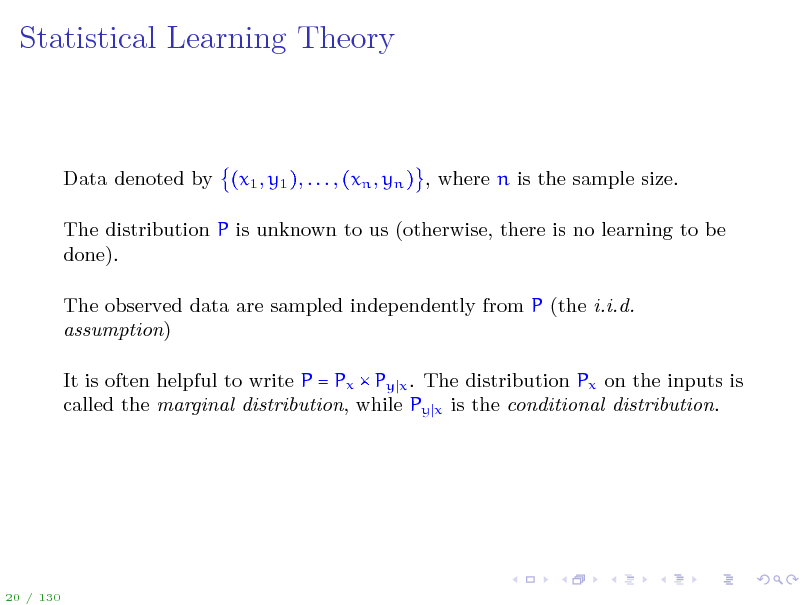
Data denoted by (x1 , y1 ), . . . , (xn , yn ) , where n is the sample size. The distribution P is unknown to us (otherwise, there is no learning to be done). The observed data are sampled independently from P (the i.i.d. assumption) It is often helpful to write P = Px Py x . The distribution Px on the inputs is called the marginal distribution, while Py x is the conditional distribution.

20 / 130

Statistical Learning Theory
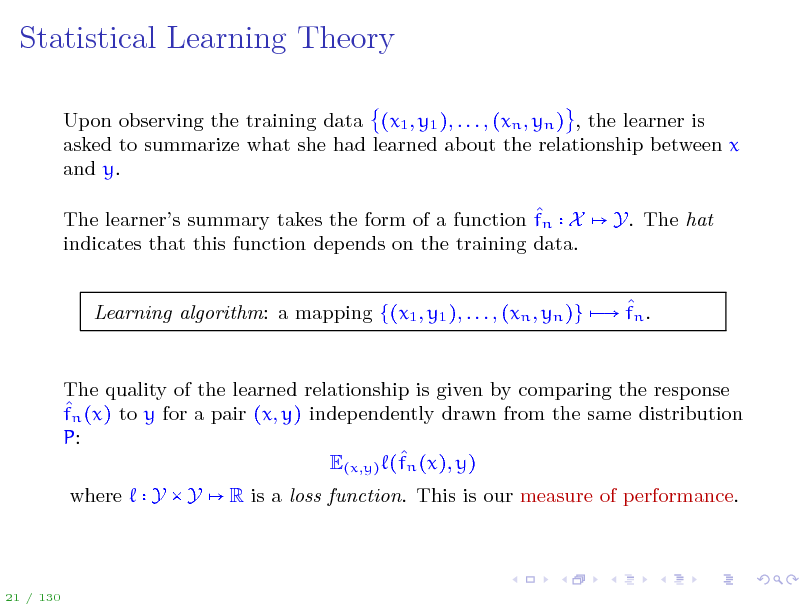
Upon observing the training data (x1 , y1 ), . . . , (xn , yn ) , the learner is asked to summarize what she had learned about the relationship between x and y. The learners summary takes the form of a function fn X indicates that this function depends on the training data. Y. The hat

Learning algorithm: a mapping {(x1 , y1 ), . . . , (xn , yn )} fn .

The quality of the learned relationship is given by comparing the response fn (x) to y for a pair (x, y) independently drawn from the same distribution P: E(x,y) (fn (x), y) where Y Y R is a loss function. This is our measure of performance.

21 / 130

Loss Functions

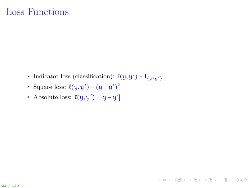
Indicator loss (classication): (y, y ) = I{yy } Square loss: (y, y ) = (y y )2 Absolute loss: (y, y ) = y y

22 / 130

Examples
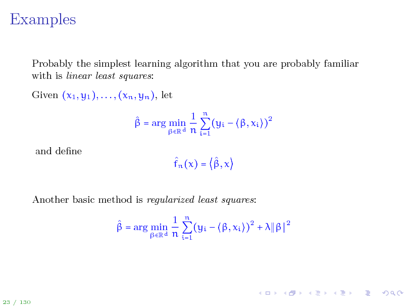
Probably the simplest learning algorithm that you are probably familiar with is linear least squares: Given (x1 , y1 ), . . . , (xn , yn ), let 1 n = arg min (yi , xi )2 Rd n i=1 and dene fn (x) = , x Another basic method is regularized least squares: 1 n = arg min (yi , xi )2 + Rd n i=1
2

23 / 130

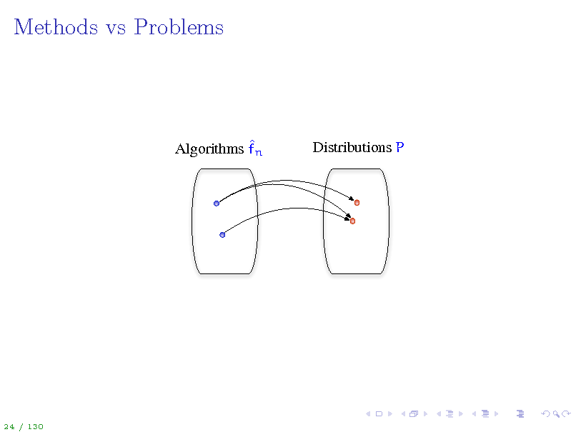
Methods vs Problems

Algorithms fn

Distributions P

24 / 130

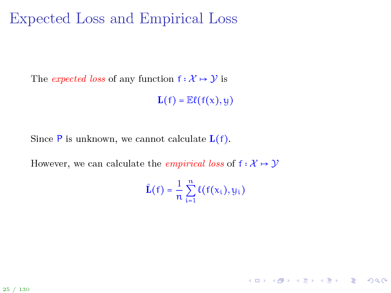
Expected Loss and Empirical Loss

The expected loss of any function f X

Y is

L(f) = E (f(x), y)

Since P is unknown, we cannot calculate L(f). However, we can calculate the empirical loss of f X 1 n L(f) = (f(xi ), yi ) n i=1 Y

25 / 130

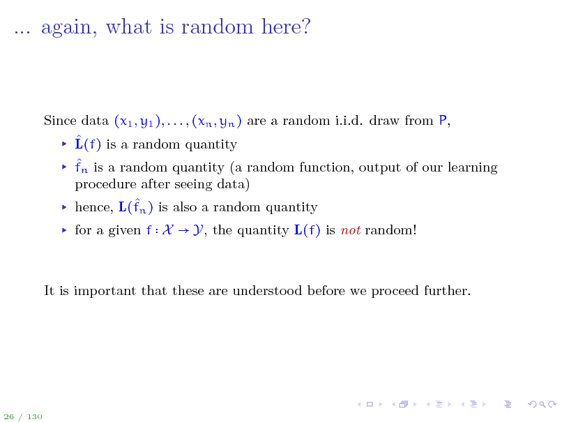
... again, what is random here?

Since data (x1 , y1 ), . . . , (xn , yn ) are a random i.i.d. draw from P, L(f) is a random quantity fn is a random quantity (a random function, output of our learning procedure after seeing data) hence, L(fn ) is also a random quantity for a given f X Y, the quantity L(f) is not random!

It is important that these are understood before we proceed further.

26 / 130

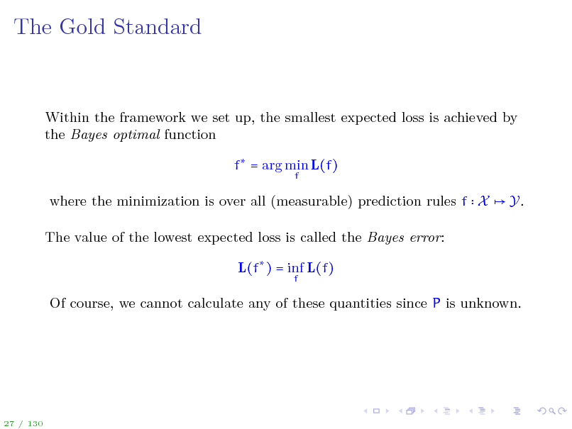
The Gold Standard

Within the framework we set up, the smallest expected loss is achieved by the Bayes optimal function f = arg min L(f)
f

where the minimization is over all (measurable) prediction rules f X The value of the lowest expected loss is called the Bayes error: L(f ) = inf L(f)
f

Y.

Of course, we cannot calculate any of these quantities since P is unknown.

27 / 130

Bayes Optimal Function
Bayes optimal function f takes on the following forms in these two particular cases: Binary classication (Y = {0, 1}) with the indicator loss: f (x) = I{(x)1
1 (x) 0
2} ,

where

(x) = E[Y X = x]

28 / 130

Bayes Optimal Function
Bayes optimal function f takes on the following forms in these two particular cases: Binary classication (Y = {0, 1}) with the indicator loss: f (x) = I{(x)1
1 (x) 0
2} ,

where

(x) = E[Y X = x]

Regression (Y = R) with squared loss: f (x) = (x), where (x) = E[Y X = x]

28 / 130

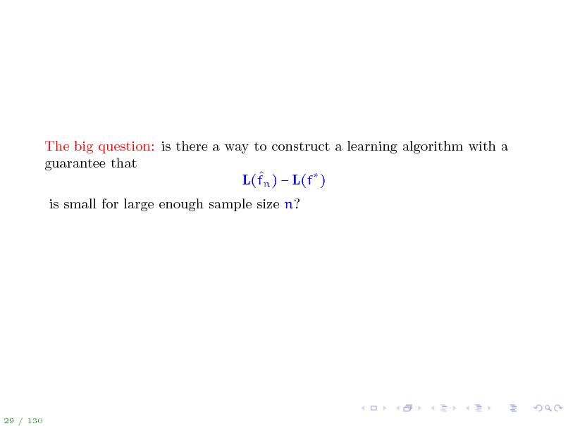
The big question: is there a way to construct a learning algorithm with a guarantee that L(fn ) L(f ) is small for large enough sample size n?

29 / 130

Outline
Introduction Statistical Learning Theory The Setting of SLT Consistency, No Free Lunch Theorems, Bias-Variance Tradeo Tools from Probability, Empirical Processes From Finite to Innite Classes Uniform Convergence, Symmetrization, and Rademacher Complexity Large Margin Theory for Classication Properties of Rademacher Complexity Covering Numbers and Scale-Sensitive Dimensions Faster Rates Model Selection Sequential Prediction / Online Learning Motivation Supervised Learning Online Convex and Linear Optimization Online-to-Batch Conversion, SVM optimization

30 / 130

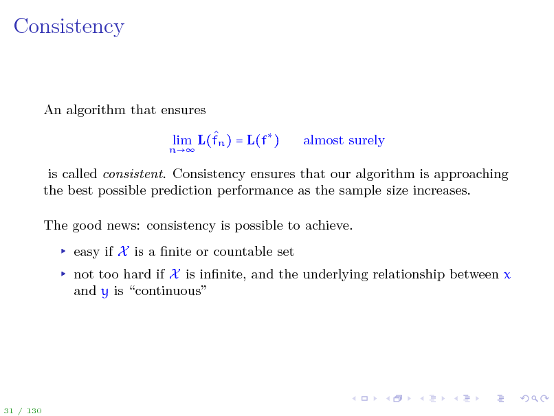
Consistency

An algorithm that ensures
n

lim L(fn ) = L(f )

almost surely

is called consistent. Consistency ensures that our algorithm is approaching the best possible prediction performance as the sample size increases. The good news: consistency is possible to achieve. easy if X is a nite or countable set not too hard if X is innite, and the underlying relationship between x and y is continuous

31 / 130

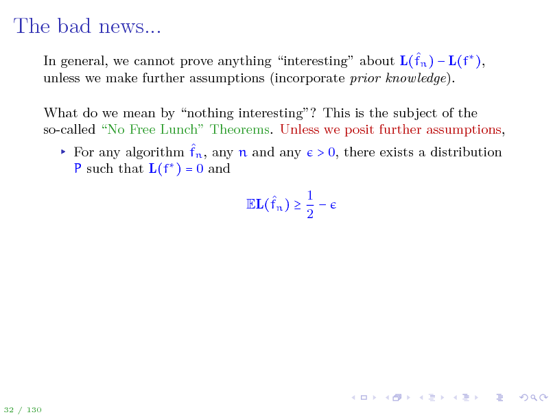
The bad news...
In general, we cannot prove anything interesting about L(fn ) L(f ), unless we make further assumptions (incorporate prior knowledge). What do we mean by nothing interesting? This is the subject of the so-called No Free Lunch Theorems. Unless we posit further assumptions,

32 / 130

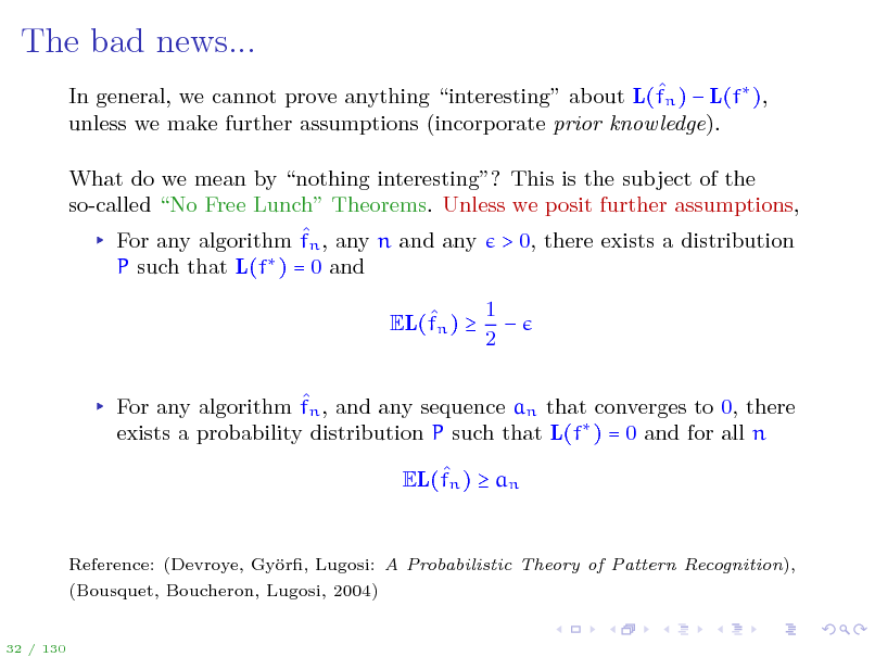
The bad news...
In general, we cannot prove anything interesting about L(fn ) L(f ), unless we make further assumptions (incorporate prior knowledge). What do we mean by nothing interesting? This is the subject of the so-called No Free Lunch Theorems. Unless we posit further assumptions, For any algorithm fn , any n and any > 0, there exists a distribution P such that L(f ) = 0 and EL(fn ) 1 2

32 / 130

The bad news...
In general, we cannot prove anything interesting about L(fn ) L(f ), unless we make further assumptions (incorporate prior knowledge). What do we mean by nothing interesting? This is the subject of the so-called No Free Lunch Theorems. Unless we posit further assumptions, For any algorithm fn , any n and any > 0, there exists a distribution P such that L(f ) = 0 and EL(fn ) 1 2

For any algorithm fn , and any sequence an that converges to 0, there exists a probability distribution P such that L(f ) = 0 and for all n EL(fn ) an

Reference: (Devroye, Gyr, Lugosi: A Probabilistic Theory of Pattern Recognition), o (Bousquet, Boucheron, Lugosi, 2004)

32 / 130

is this really bad news?

Not really. We always have some domain knowledge. Two ways of incorporating prior knowledge: Direct way: assume that the distribution P is not arbitrary (also known as a modeling approach, generative approach, statistical modeling) Indirect way: redene the goal to perform as well as a reference set F of predictors: L(fn ) inf L(f)
fF

This is known as a discriminative approach. F encapsulates our inductive bias.

33 / 130

Pros/Cons of the two approaches
Pros of the discriminative approach: we never assume that P takes some particular form, but we rather put our prior knowledge into what are the types of predictors that will do well. Cons: cannot really interpret fn .

Pros of the generative approach: can estimate the model / parameters of the distribution (inference). Cons: it is not clear what the analysis says if the assumption is actually violated.

Both approaches have their advantages. A machine learning researcher or practitioner should ideally know both and should understand their strengths and weaknesses. In this tutorial we only focus on the discriminative approach.

34 / 130

Example: Linear Discriminant Analysis
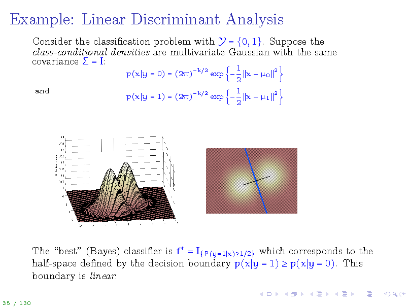
Consider the classication problem with Y = {0, 1}. Suppose the class-conditional densities are multivariate Gaussian with the same covariance = I:
p(x y = 0) = (2) and p(x y = 1) = (2)
k 2 k

1 x 0 2 1 2 exp x 1 2 exp

2

2

The best (Bayes) classier is f = I{P(y=1 x)1 2} which corresponds to the half-space dened by the decision boundary p(x y = 1) p(x y = 0). This boundary is linear.
35 / 130

Example: Linear Discriminant Analysis
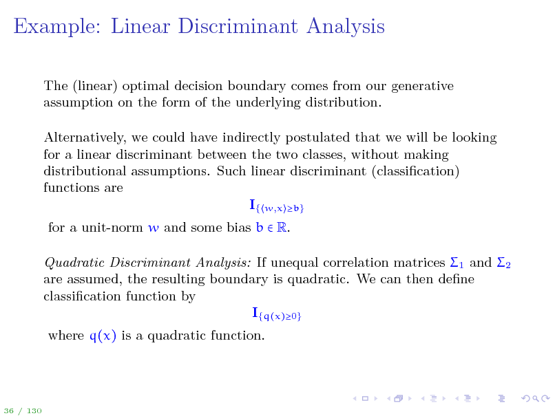
The (linear) optimal decision boundary comes from our generative assumption on the form of the underlying distribution. Alternatively, we could have indirectly postulated that we will be looking for a linear discriminant between the two classes, without making distributional assumptions. Such linear discriminant (classication) functions are I{ w,x b} for a unit-norm w and some bias b R. Quadratic Discriminant Analysis: If unequal correlation matrices 1 and 2 are assumed, the resulting boundary is quadratic. We can then dene classication function by I{q(x)0} where q(x) is a quadratic function.

36 / 130

Bias-Variance Tradeo
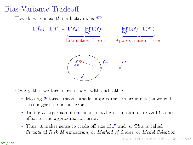
How do we choose the inductive bias F? L(fn ) L(f ) = L(fn ) inf L(f)
fF

+

fF

inf L(f) L(f )

Estimation Error

Approximation Error

fn F

fF

f

Clearly, the two terms are at odds with each other: Making F larger means smaller approximation error but (as we will see) larger estimation error Taking a larger sample n means smaller estimation error and has no eect on the approximation error. Thus, it makes sense to trade o size of F and n. This is called Structural Risk Minimization, or Method of Sieves, or Model Selection.
37 / 130

Bias-Variance Tradeo

We will only focus on the estimation error, yet the ideas we develop will make it possible to read about model selection on your own. Note: if we guessed correctly and f F, then L(fn ) L(f ) = L(fn ) inf L(f)
fF

For a particular problem, one hopes that prior knowledge about the problem can ensure that the approximation error inf fF L(f) L(f ) is small.

38 / 130

Occams Razor

Occams Razor is often quoted as a principle for choosing the simplest theory or explanation out of the possible ones. However, this is a rather philosophical argument since simplicity is not uniquely dened. We will discuss this issue later. What we will do is to try to understand complexity when it comes to behavior of certain stochastic processes. Such a question will be well-dened mathematically.

39 / 130

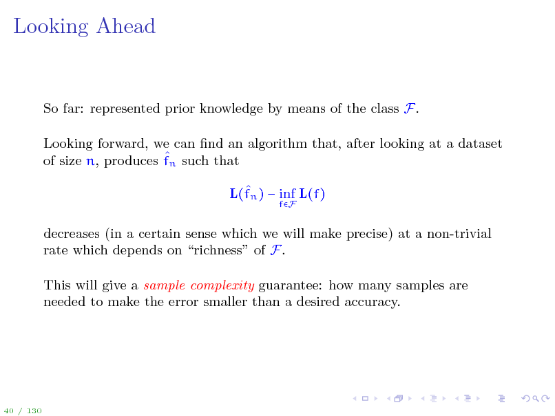
Looking Ahead

So far: represented prior knowledge by means of the class F. Looking forward, we can nd an algorithm that, after looking at a dataset of size n, produces fn such that L(fn ) inf L(f)
fF

decreases (in a certain sense which we will make precise) at a non-trivial rate which depends on richness of F. This will give a sample complexity guarantee: how many samples are needed to make the error smaller than a desired accuracy.

40 / 130

Outline
Introduction Statistical Learning Theory The Setting of SLT Consistency, No Free Lunch Theorems, Bias-Variance Tradeo Tools from Probability, Empirical Processes From Finite to Innite Classes Uniform Convergence, Symmetrization, and Rademacher Complexity Large Margin Theory for Classication Properties of Rademacher Complexity Covering Numbers and Scale-Sensitive Dimensions Faster Rates Model Selection Sequential Prediction / Online Learning Motivation Supervised Learning Online Convex and Linear Optimization Online-to-Batch Conversion, SVM optimization

41 / 130

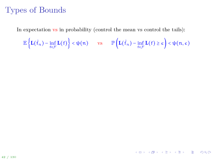
Types of Bounds
In expectation vs in probability (control the mean vs control the tails): E L(fn ) inf L(f) < (n)
fF

vs

P L(fn ) inf L(f)
fF

< (n, )

42 / 130

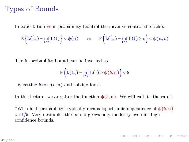
Types of Bounds
In expectation vs in probability (control the mean vs control the tails): E L(fn ) inf L(f) < (n)
fF

vs

P L(fn ) inf L(f)
fF

< (n, )

The in-probability bound can be inverted as P L(fn ) inf L(f) (, n) <
fF

by setting = ( , n) and solving for . In this lecture, we are after the function (, n). We will call it the rate. With high probability typically means logarithmic dependence of (, n) on 1 . Very desirable: the bound grows only modestly even for high condence bounds.

42 / 130

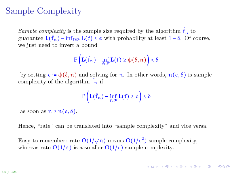
Sample Complexity
Sample complexity is the sample size required by the algorithm fn to guarantee L(fn ) inf fF L(f) with probability at least 1 . Of course, we just need to invert a bound P L(fn ) inf L(f) (, n) <
fF

by setting = (, n) and solving for n. In other words, n( , ) is sample complexity of the algorithm fn if P L(fn ) inf L(f)
fF

as soon as n n( , ). Hence, rate can be translated into sample complexity and vice versa. Easy to remember: rate O(1 n) means O(1 2 ) sample complexity, whereas rate O(1 n) is a smaller O(1 ) sample complexity.

43 / 130

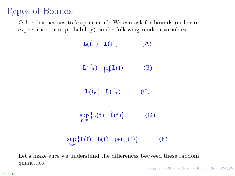
Types of Bounds
Other distinctions to keep in mind: We can ask for bounds (either in expectation or in probability) on the following random variables: L(fn ) L(f ) (A)

L(fn ) inf L(f)
fF

(B)

L(fn ) L(fn )

(C)

sup L(f) L(f)
fF

(D)

sup L(f) L(f) penn (f)
fF

(E)

Lets make sure we understand the dierences between these random quantities!
44 / 130

Types of Bounds
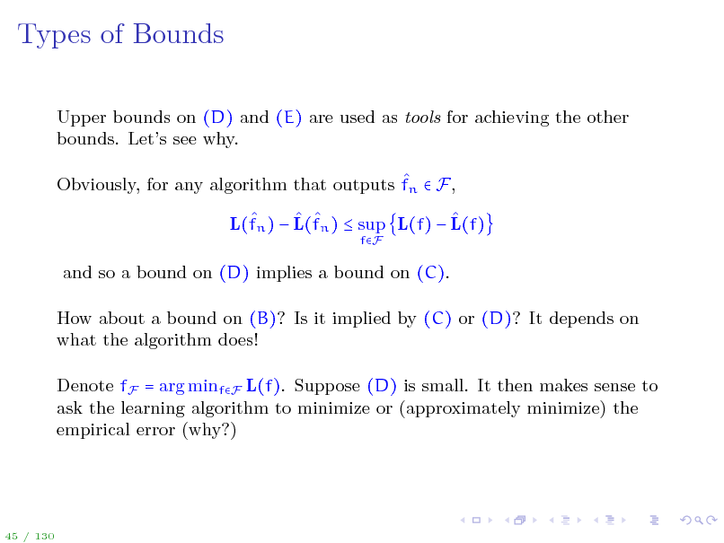
Upper bounds on (D) and (E) are used as tools for achieving the other bounds. Lets see why. Obviously, for any algorithm that outputs fn F, L(fn ) L(fn ) sup L(f) L(f)
fF

and so a bound on (D) implies a bound on (C). How about a bound on (B)? Is it implied by (C) or (D)? It depends on what the algorithm does! Denote fF = arg minfF L(f). Suppose (D) is small. It then makes sense to ask the learning algorithm to minimize or (approximately minimize) the empirical error (why?)

45 / 130

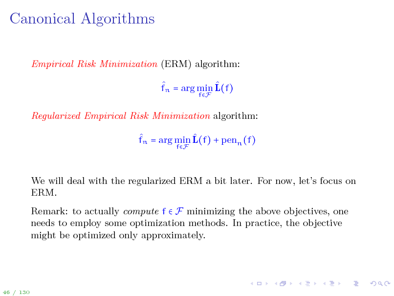
Canonical Algorithms
Empirical Risk Minimization (ERM) algorithm: fn = arg min L(f)
fF

Regularized Empirical Risk Minimization algorithm: fn = arg min L(f) + penn (f)
fF

We will deal with the regularized ERM a bit later. For now, lets focus on ERM. Remark: to actually compute f F minimizing the above objectives, one needs to employ some optimization methods. In practice, the objective might be optimized only approximately.

46 / 130

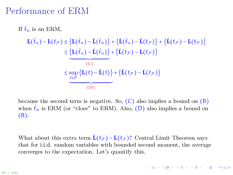
Performance of ERM
If fn is an ERM, L(fn ) L(fF ) L(fn ) L(fn ) + L(fn ) L(fF ) + L(fF ) L(fF ) L(fn ) L(fn ) + L(fF ) L(fF )
(C)

sup L(f) L(f) + L(fF ) L(fF )
fF (D)

because the second term is negative. So, (C) also implies a bound on (B) when fn is ERM (or close to ERM). Also, (D) also implies a bound on (B). What about this extra term L(fF ) L(fF )? Central Limit Theorem says that for i.i.d. random variables with bounded second moment, the average converges to the expectation. Lets quantify this.

47 / 130

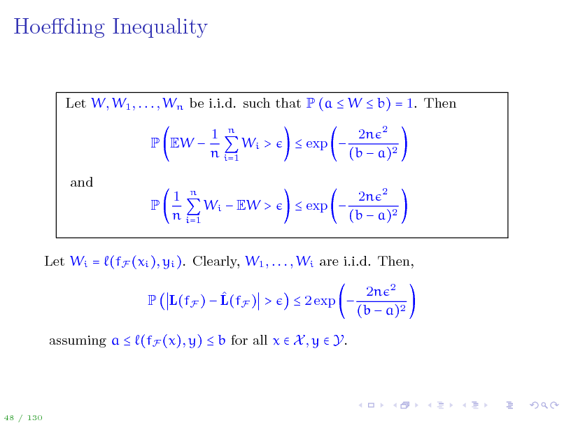
Hoeding Inequality

Let W, W1 , . . . , Wn be i.i.d. such that P (a W b) = 1. Then P EW and P 1 n Wi > n i=1 exp 2n 2 (b a)2 2n 2 (b a)2

1 n Wi EW > n i=1

exp

Let Wi = (fF (xi ), yi ). Clearly, W1 , . . . , Wi are i.i.d. Then, P L(fF ) L(fF ) > 2 exp 2n 2 (b a)2

assuming a (fF (x), y) b for all x X , y Y.

48 / 130

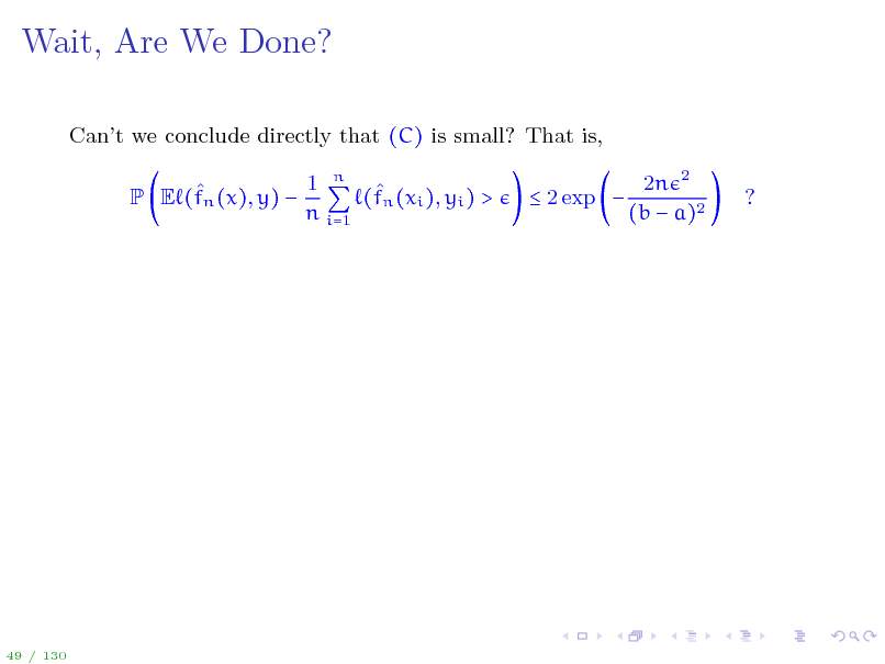
Wait, Are We Done?
Cant we conclude directly that (C) is small? That is, P E (fn (x), y) 1 n (fn (xi ), yi ) > n i=1 2 exp 2n 2 (b a)2 ?

49 / 130

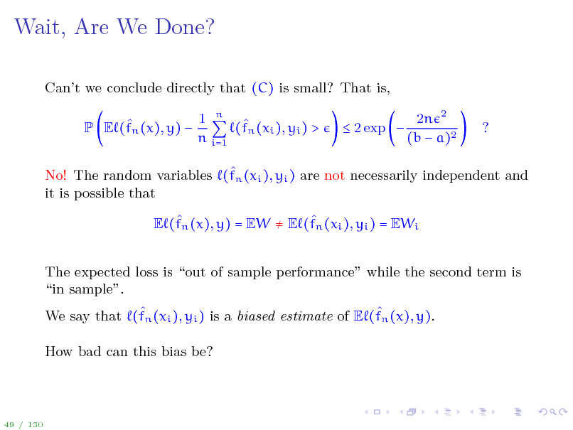
Wait, Are We Done?
Cant we conclude directly that (C) is small? That is, P E (fn (x), y) 1 n (fn (xi ), yi ) > n i=1 2 exp 2n 2 (b a)2 ?

No! The random variables (fn (xi ), yi ) are not necessarily independent and it is possible that E (fn (x), y) = EW E (fn (xi ), yi ) = EWi The expected loss is out of sample performance while the second term is in sample. We say that (fn (xi ), yi ) is a biased estimate of E (fn (x), y). How bad can this bias be?

49 / 130

Example
X = [0, 1], Y = {0, 1} (f(Xi ), Yi ) = I{f(Xi )Yi } distribution P = Px Py x with Px = Unif[0, 1] and Py x = y=1 function class F = nN f = fS S X , S = n, fS (x) = I{xS}

1 0 1

ERM fn memorizes (perfectly ts) the data, but has no ability to generalize. Observe that 0 = E (fn (xi ), yi ) E (fn (x), y) = 1 This phenomenon is called overtting.
50 / 130

Example
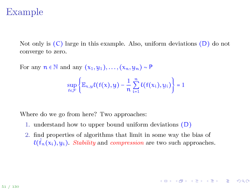
Not only is (C) large in this example. Also, uniform deviations (D) do not converge to zero. For any n N and any (x1 , y1 ), . . . , (xn , yn ) P sup Ex,y (f(x), y)
fF

1 n (f(xi ), yi ) = 1 n i=1

Where do we go from here? Two approaches: 1. understand how to upper bound uniform deviations (D) 2. nd properties of algorithms that limit in some way the bias of (fn (xi ), yi ). Stability and compression are two such approaches.

51 / 130

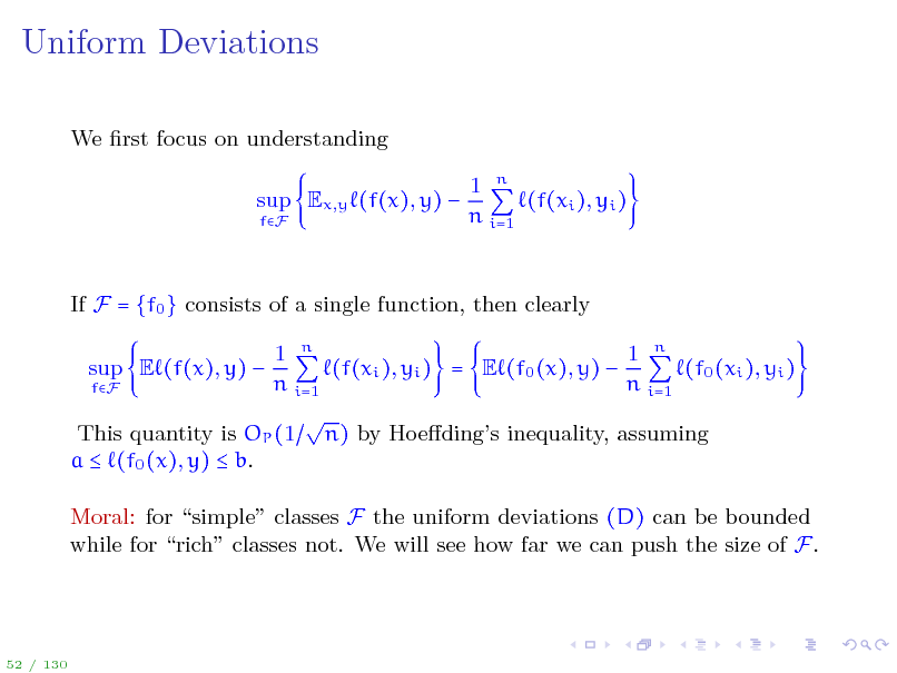
Uniform Deviations
We rst focus on understanding sup Ex,y (f(x), y)
fF

1 n (f(xi ), yi ) n i=1

If F = {f0 } consists of a single function, then clearly sup E (f(x), y)
fF

1 n 1 n (f(xi ), yi ) = E (f0 (x), y) (f0 (xi ), yi ) n i=1 n i=1 n) by Hoedings inequality, assuming

This quantity is OP (1 a (f0 (x), y) b.

Moral: for simple classes F the uniform deviations (D) can be bounded while for rich classes not. We will see how far we can push the size of F.

52 / 130

A bit of notation to simplify things...
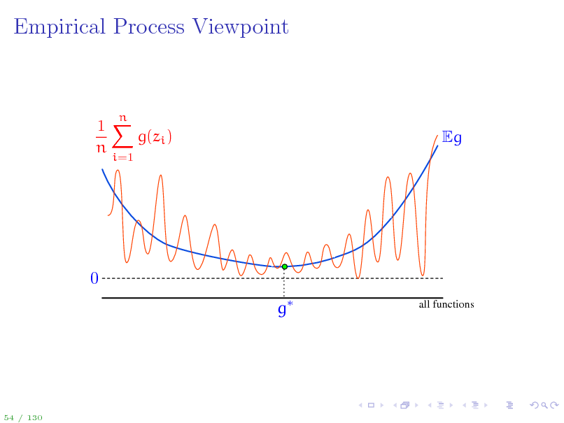
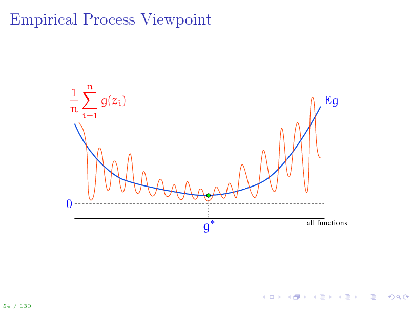
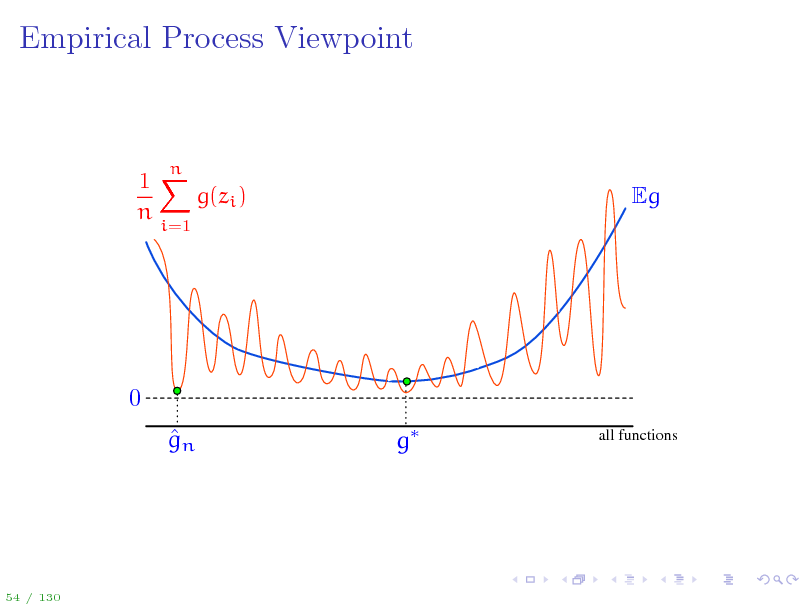
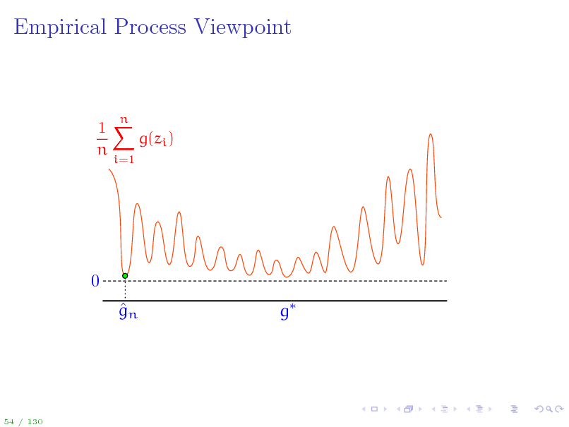
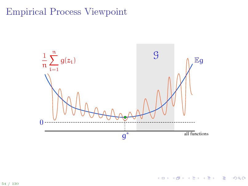
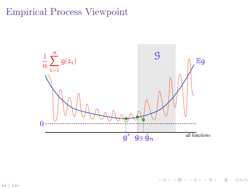
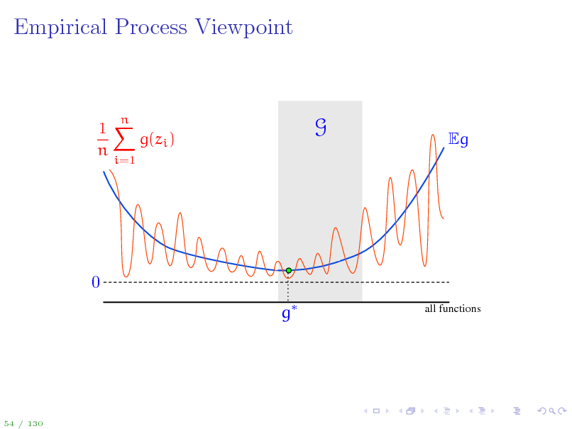
To ease the notation, Let zi = (xi , yi ) so that the training data is {z1 , . . . , zn } g(z) = (f(x), y) for z = (x, y) Loss class G = g g(z) = (f(x), y) = F gn = (fn (), ), gG = (fF (), ) g = arg ming Eg(z) = (f (), ) is Bayes optimal (loss) function We can now work with the set G, but keep in mind that each g G corresponds to an f F: g G f F Once again, the quantity of interest is sup Eg(z)
gG

1 n g(zi ) n i=1

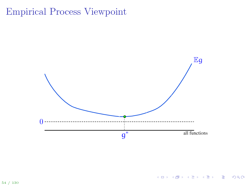
1 On the next slide, we visualize deviations Eg(z) n n g(zi ) for all i=1 possible functions g and discuss all the concepts introduces so far.

53 / 130

Empirical Process Viewpoint

Eg

0 g
all functions

54 / 130

Empirical Process Viewpoint

1X g(zi ) n
i=1

n

Eg

0 g
all functions

54 / 130

Empirical Process Viewpoint

1X g(zi ) n
i=1

n

Eg

0 g
all functions

54 / 130

Empirical Process Viewpoint

1X g(zi ) n
i=1

n

Eg

0 gn g
all functions

54 / 130

Empirical Process Viewpoint

1X g(zi ) n
i=1

n

0 gn g

54 / 130

Empirical Process Viewpoint

1X g(zi ) n
i=1

n

G

Eg

0 g
all functions

54 / 130

Empirical Process Viewpoint

1X g(zi ) n
i=1

n

G

Eg

0 g gG gn
all functions

54 / 130

Empirical Process Viewpoint

1X g(zi ) n
i=1

n

G

Eg

0 g
all functions

54 / 130

Empirical Process Viewpoint
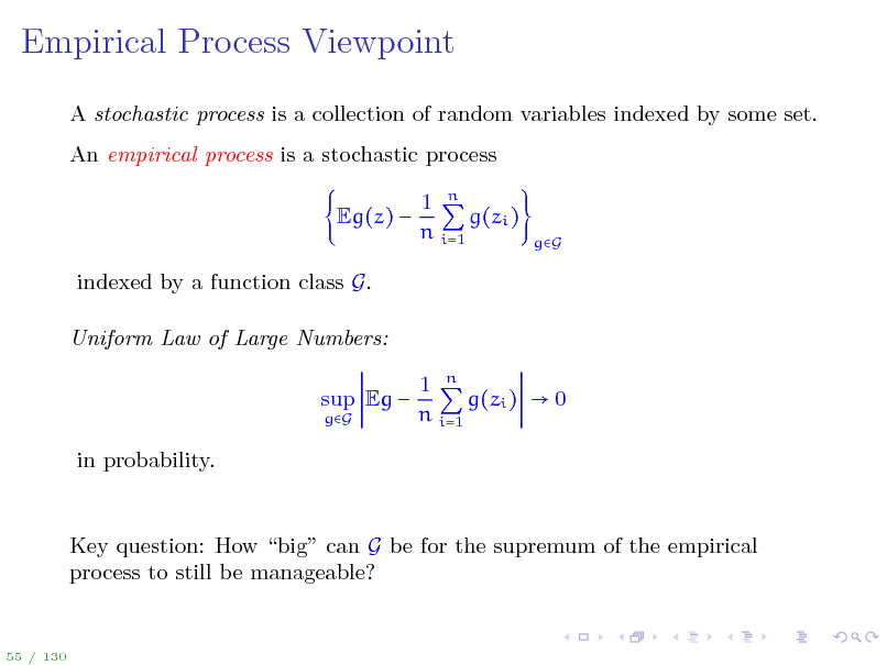
A stochastic process is a collection of random variables indexed by some set. An empirical process is a stochastic process Eg(z) indexed by a function class G. Uniform Law of Large Numbers: sup Eg
gG

1 n g(zi ) n i=1

gG

1 n g(zi ) 0 n i=1

in probability.

55 / 130

Empirical Process Viewpoint
A stochastic process is a collection of random variables indexed by some set. An empirical process is a stochastic process Eg(z) indexed by a function class G. Uniform Law of Large Numbers: sup Eg
gG

1 n g(zi ) n i=1

gG

1 n g(zi ) 0 n i=1

in probability.

Key question: How big can G be for the supremum of the empirical process to still be manageable?

55 / 130

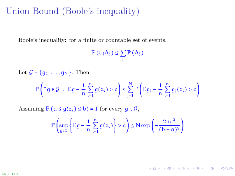
Union Bound (Booles inequality)
Booles inequality: for a nite or countable set of events, P (j Aj )
j

P (Aj )

Let G = {g1 , . . . , gN }. Then P g G Eg 1 n g(zi ) > n i=1
N j=1

P Egj

1 n gj (zi ) > n i=1

Assuming P (a g(zi ) b) = 1 for every g G, P sup Eg
gG

1 n g(zi ) > n i=1

N exp

2n 2 (b a)2

56 / 130

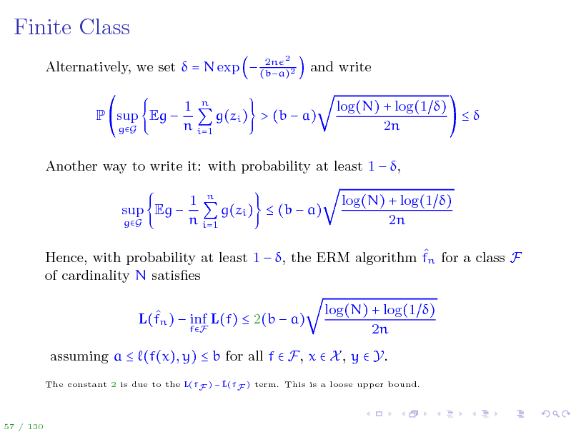
Finite Class
2n Alternatively, we set = N exp (ba)2
2

and write log(N) + log(1 ) 2n

P sup Eg
gG

1 n g(zi ) > (b a) n i=1

Another way to write it: with probability at least 1 , sup Eg
gG

1 n g(zi ) (b a) n i=1

log(N) + log(1 ) 2n

Hence, with probability at least 1 , the ERM algorithm fn for a class F of cardinality N satises L(fn ) inf L(f) 2(b a)
fF

log(N) + log(1 ) 2n

assuming a (f(x), y) b for all f F, x X , y Y.
The constant 2 is due to the L(fF ) F ) term. This is a loose upper bound. L(f

57 / 130

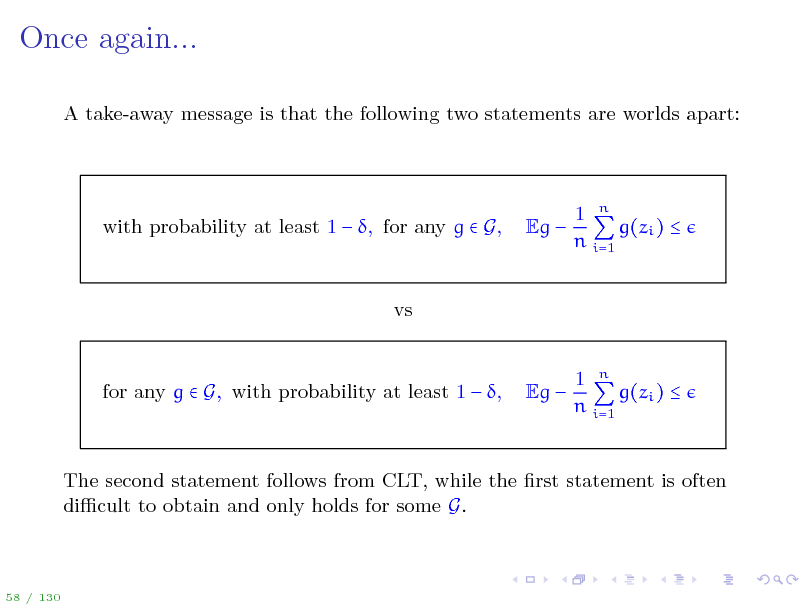
Once again...
A take-away message is that the following two statements are worlds apart:

with probability at least 1 , for any g G,

Eg

1 n g(zi ) n i=1

vs 1 n g(zi ) n i=1

for any g G, with probability at least 1 ,

Eg

The second statement follows from CLT, while the rst statement is often dicult to obtain and only holds for some G.

58 / 130

Outline
Introduction Statistical Learning Theory The Setting of SLT Consistency, No Free Lunch Theorems, Bias-Variance Tradeo Tools from Probability, Empirical Processes From Finite to Innite Classes Uniform Convergence, Symmetrization, and Rademacher Complexity Large Margin Theory for Classication Properties of Rademacher Complexity Covering Numbers and Scale-Sensitive Dimensions Faster Rates Model Selection Sequential Prediction / Online Learning Motivation Supervised Learning Online Convex and Linear Optimization Online-to-Batch Conversion, SVM optimization

59 / 130

Countable Class: Weighted Union Bound
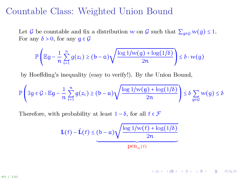
Let G be countable and x a distribution w on G such that gG w(g) 1. For any > 0, for any g G P Eg 1 n g(zi ) (b a) n i=1 log 1 w(g) + log(1 ) w(g) 2n

by Hoedings inequality (easy to verify!). By the Union Bound, P g G Eg 1 n g(zi ) (b a) n i=1 log 1 w(g) + log(1 ) w(g) 2n gG

Therefore, with probability at least 1 , for all f F L(f) L(f) (b a) log 1 w(f) + log(1 ) 2n penn (f)

60 / 130

Countable Class: Weighted Union Bound
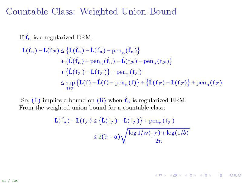
If fn is a regularized ERM, L(fn ) L(fF ) L(fn ) L(fn ) penn (fn ) + L(fn ) + penn (fn ) L(fF ) penn (fF ) + L(fF ) L(fF ) + penn (fF ) sup L(f) L(f) penn (f) + L(fF ) L(fF ) + penn (fF )
fF

So, (E) implies a bound on (B) when fn is regularized ERM. From the weighted union bound for a countable class: L(fn ) L(fF ) L(fF ) L(fF ) + penn (fF ) 2(b a) log 1 w(fF ) + log(1 ) 2n

61 / 130

Uncountable Class: Compression Bounds
Let us make the dependence of the algorithm fn on the training set n = fn [S]. S = {(x1 , y1 ), . . . , (xn , yn )} explicit: f Suppose F has the property that there exists a compression function Ck which selects from any dataset S of any size n a subset of k labeled examples Ck (S) S such that the algorithm can be written as fn [S] = fk [Ck (S)] Then, 1 n (fk [Ck (S)](xi ), yi ) L(fn ) L(fn ) = E (fk [Ck (S)](x), y) n i=1
I{1,...,n}, I k

max

1 n E (fk [SI ](x), y) (fk [SI ](xi ), yi ) n i=1

62 / 130

Uncountable Class: Compression Bounds
Since fk [SI ] only depends on k out of n points, the empirical average is mostly out of sample. Adding and subtracting 1 (fk [SI ](x ), y ) n (x ,y )W
for an additional set of i.i.d. random variables W = {(x1 , y1 ), . . . , (xk , yk )} results in an upper bound

I{1,...,n}, I k

max

1 E (fk [SI ](x), y) n (x,y)S

SI W I

(fk [SI ](x), y) +

(b a)k n

We appeal to the union bound over the n possibilities, with a Hoedings k bound for each. Then with probability at least 1 , L(fn ) inf L(f) 2(b a)
fF

k log(en k) + log(1 ) (b a)k + 2n n

assuming a (f(x), y) b for all f F, x X , y Y.
63 / 130

Example: Classication with Thresholds in 1D
X = [0, 1], Y = {0, 1} F = f f (x) = I{x} , [0, 1] (f (x), y) = I{f (x)y}

fn 0 1

For any set of data (x1 , y1 ), . . . , (xn , yn ), the ERM solution fn has the property that the rst occurrence xl on the left of the threshold has label yl = 0, while rst occurrence xr on the right label yr = 1. Enough to take k = 2 and dene fn [S] = f2 [(xl , 0), (xr , 1)].

64 / 130

Stability
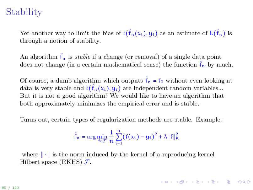
Yet another way to limit the bias of (fn (xi ), yi ) as an estimate of L(fn ) is through a notion of stability. An algorithm fn is stable if a change (or removal) of a single data point does not change (in a certain mathematical sense) the function fn by much. Of course, a dumb algorithm which outputs fn = f0 without even looking at n (xi ), yi ) are independent random variables... data is very stable and (f But it is not a good algorithm! We would like to have an algorithm that both approximately minimizes the empirical error and is stable. Turns out, certain types of regularization methods are stable. Example: 1 n fn = arg min (f(xi ) yi )2 + f fF n i=1
2 K

where is the norm induced by the kernel of a reproducing kernel Hilbert space (RKHS) F.

65 / 130

Summary so far

We proved upper bounds on L(fn ) L(fF ) for ERM over a nite class Regularized ERM over a countable class (weighted union bound) ERM over classes F with the compression property ERM or Regularized ERM that are stable (only sketched it) What about a more general situation? Is there a way to measure complexity of F that tells us whether ERM will succeed?

66 / 130

Outline
Introduction Statistical Learning Theory The Setting of SLT Consistency, No Free Lunch Theorems, Bias-Variance Tradeo Tools from Probability, Empirical Processes From Finite to Innite Classes Uniform Convergence, Symmetrization, and Rademacher Complexity Large Margin Theory for Classication Properties of Rademacher Complexity Covering Numbers and Scale-Sensitive Dimensions Faster Rates Model Selection Sequential Prediction / Online Learning Motivation Supervised Learning Online Convex and Linear Optimization Online-to-Batch Conversion, SVM optimization

67 / 130

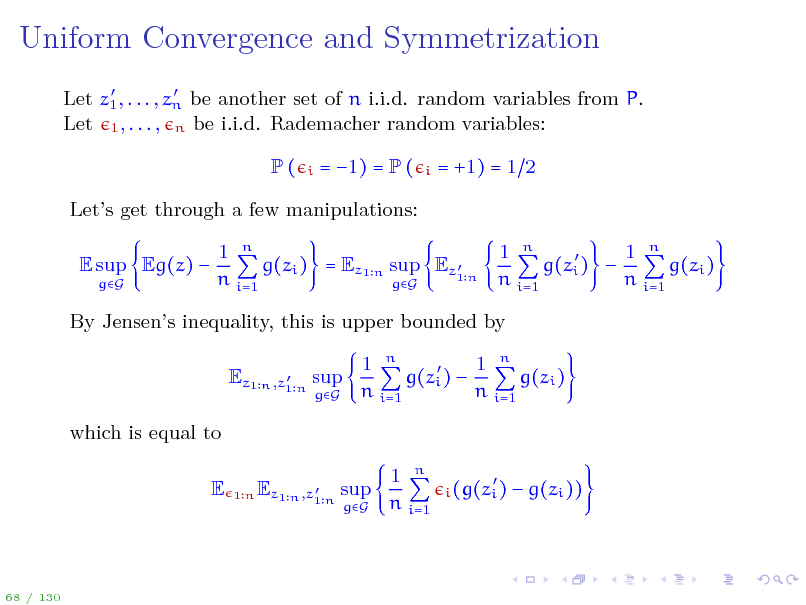
Uniform Convergence and Symmetrization
Let z1 , . . . , zn be another set of n i.i.d. random variables from P. Let 1 , . . . , n be i.i.d. Rademacher random variables:

P(

i

= 1) = P (

i

= +1) = 1 2

Lets get through a few manipulations: E sup Eg(z)
gG

1 n 1 n 1 n g(zi ) = Ez1 n sup Ez1 n g(zi ) g(zi ) n i=1 n i=1 n i=1 gG

By Jensens inequality, this is upper bounded by
Ez1 n ,z1 n sup

gG

1 n 1 n g(zi ) g(zi ) n i=1 n i=1

which is equal to E
1n Ez1 n ,z1 n sup

gG

1 n n i=1

i (g(zi )

g(zi ))

68 / 130

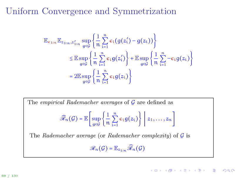
Uniform Convergence and Symmetrization
E
Ez1 n ,z1 n sup

1n

gG

1 n n i=1 1 n n i=1 1 n i=1
n

i (g(zi ) i g(zi ) i g(zi )

g(zi )) 1 n i g(zi ) n i=1

E sup
gG

+ E sup
gG

= 2E sup
gG

The empirical Rademacher averages of G are dened as Rn (G) = E sup
gG

1 n n i=1

i g(zi )

z1 , . . . , zn

The Rademacher average (or Rademacher complexity) of G is Rn (G) = Ez1 n Rn (G)

69 / 130

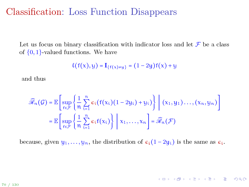
Classication: Loss Function Disappears
Let us focus on binary classication with indicator loss and let F be a class of {0, 1}-valued functions. We have (f(x), y) = I{f(x)y} = (1 2y)f(x) + y and thus 1 n n i=1 1 n n i=1

Rn (G) = E sup
fF

i (f(xi )(1 i f(xi )

2yi ) + yi )

(x1 , y1 ) . . . , (xn , yn )

= E sup
fF

x1 , . . . , xn = Rn (F)
i (1

because, given y1 , . . . , yn , the distribution of

2yi ) is the same as

i.

70 / 130

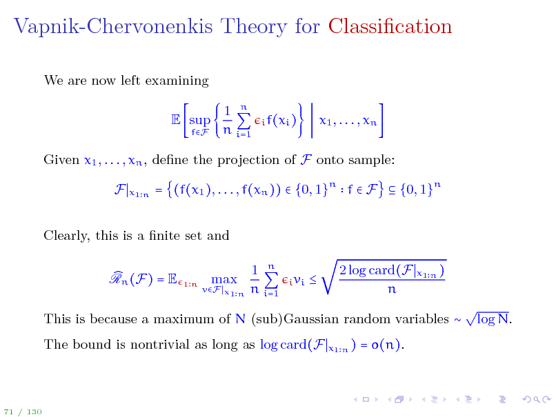
Vapnik-Chervonenkis Theory for Classication
We are now left examining E sup
fF

1 n n i=1

i f(xi )

x1 , . . . , xn

Given x1 , . . . , xn , dene the projection of F onto sample: F
x1 n

= (f(x1 ), . . . , f(xn )) {0, 1}n f F {0, 1}n

Clearly, this is a nite set and Rn (F) = E max 1 n n i=1
i vi

1n

vF x1 n

2 log card(F n

x1 n )

This is because a maximum of N (sub)Gaussian random variables The bound is nontrivial as long as log card(F
x1 n )

log N.

= o(n).

71 / 130

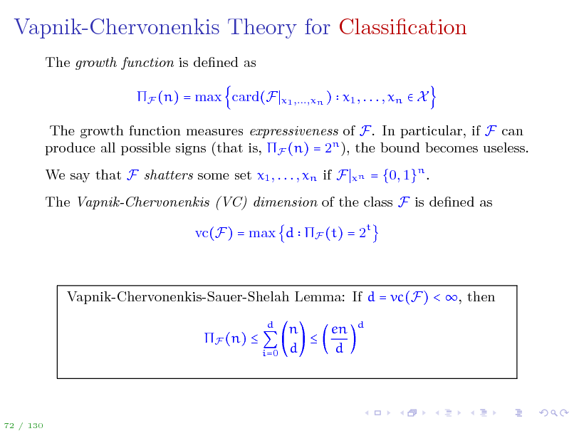
Vapnik-Chervonenkis Theory for Classication
The growth function is dened as F (n) = max card(F
x1 ,...,xn )

x1 , . . . , xn X

The growth function measures expressiveness of F. In particular, if F can produce all possible signs (that is, F (n) = 2n ), the bound becomes useless. We say that F shatters some set x1 , . . . , xn if F
xn

= {0, 1}n .

The Vapnik-Chervonenkis (VC) dimension of the class F is dened as vc(F) = max d F (t) = 2t

Vapnik-Chervonenkis-Sauer-Shelah Lemma: If d = vc(F) < , then F (n)
d i=0

n en d d

d

72 / 130

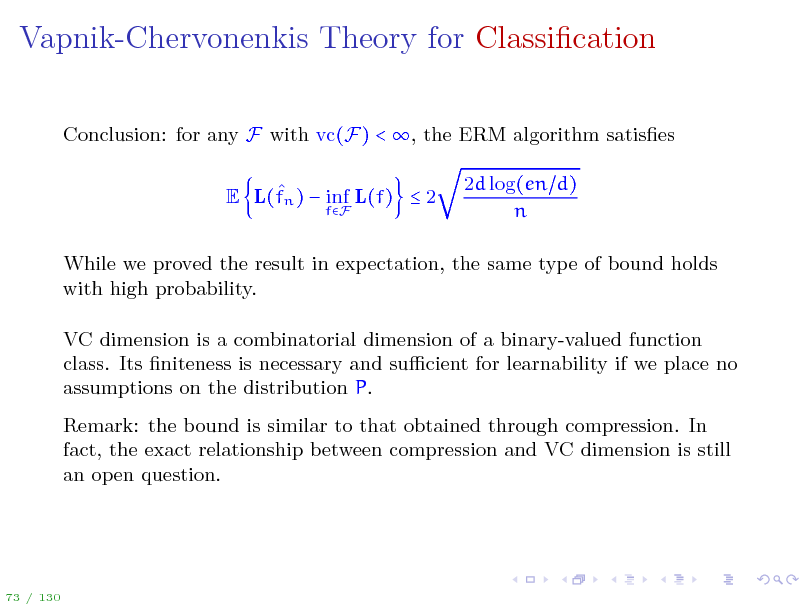
Vapnik-Chervonenkis Theory for Classication
Conclusion: for any F with vc(F) < , the ERM algorithm satises E L(fn ) inf L(f) 2
fF

2d log(en d) n

While we proved the result in expectation, the same type of bound holds with high probability. VC dimension is a combinatorial dimension of a binary-valued function class. Its niteness is necessary and sucient for learnability if we place no assumptions on the distribution P. Remark: the bound is similar to that obtained through compression. In fact, the exact relationship between compression and VC dimension is still an open question.

73 / 130

Vapnik-Chervonenkis Theory for Classication
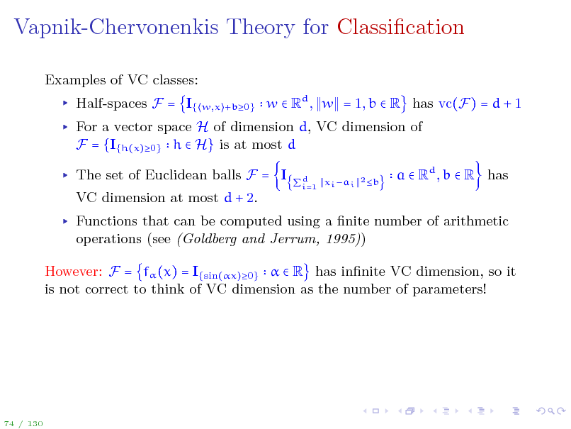
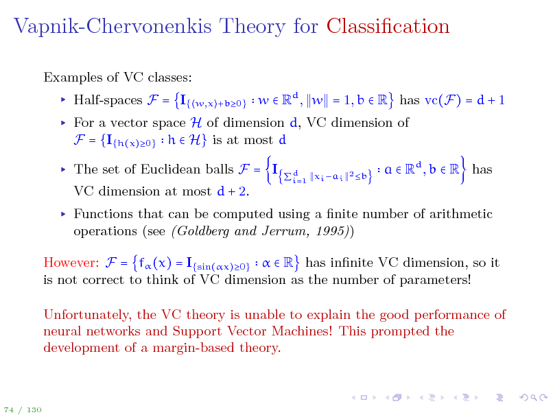
Examples of VC classes: Half-spaces F = I{
w,x +b0}

w Rd , w = 1, b R has vc(F) = d + 1

For a vector space H of dimension d, VC dimension of F = {I{h(x)0} h H} is at most d The set of Euclidean balls F = I VC dimension at most d + 2.
xi ai 2 b d i=1

a Rd , b R has

Functions that can be computed using a nite number of arithmetic operations (see (Goldberg and Jerrum, 1995)) However: F = f (x) = I{sin(x)0} R has innite VC dimension, so it is not correct to think of VC dimension as the number of parameters!

74 / 130

Vapnik-Chervonenkis Theory for Classication
Examples of VC classes: Half-spaces F = I{
w,x +b0}

w Rd , w = 1, b R has vc(F) = d + 1

For a vector space H of dimension d, VC dimension of F = {I{h(x)0} h H} is at most d The set of Euclidean balls F = I VC dimension at most d + 2.
xi ai 2 b d i=1

a Rd , b R has

Functions that can be computed using a nite number of arithmetic operations (see (Goldberg and Jerrum, 1995)) However: F = f (x) = I{sin(x)0} R has innite VC dimension, so it is not correct to think of VC dimension as the number of parameters! Unfortunately, the VC theory is unable to explain the good performance of neural networks and Support Vector Machines! This prompted the development of a margin-based theory.

74 / 130

Outline
Introduction Statistical Learning Theory The Setting of SLT Consistency, No Free Lunch Theorems, Bias-Variance Tradeo Tools from Probability, Empirical Processes From Finite to Innite Classes Uniform Convergence, Symmetrization, and Rademacher Complexity Large Margin Theory for Classication Properties of Rademacher Complexity Covering Numbers and Scale-Sensitive Dimensions Faster Rates Model Selection Sequential Prediction / Online Learning Motivation Supervised Learning Online Convex and Linear Optimization Online-to-Batch Conversion, SVM optimization

75 / 130

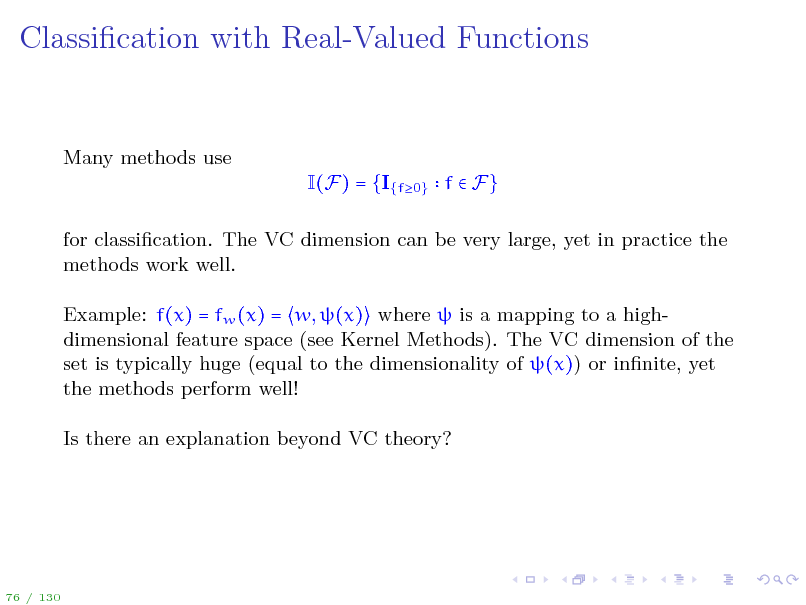
Classication with Real-Valued Functions

Many methods use I(F) = {I{f0} f F} for classication. The VC dimension can be very large, yet in practice the methods work well. Example: f(x) = fw (x) = w, (x) where is a mapping to a highdimensional feature space (see Kernel Methods). The VC dimension of the set is typically huge (equal to the dimensionality of (x)) or innite, yet the methods perform well! Is there an explanation beyond VC theory?

76 / 130

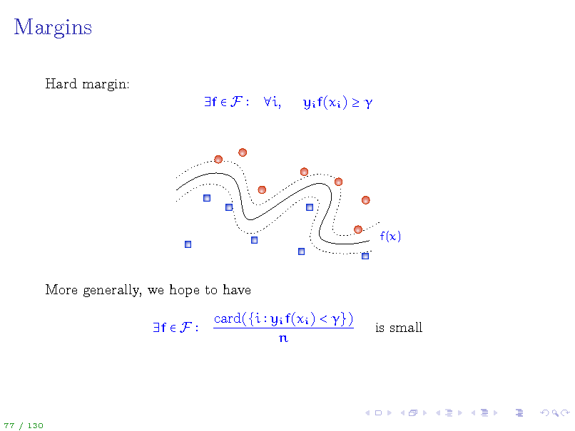
Margins
Hard margin: f F i, yi f(xi )

f(x)

More generally, we hope to have f F card({i yi f(xi ) < }) n is small

77 / 130

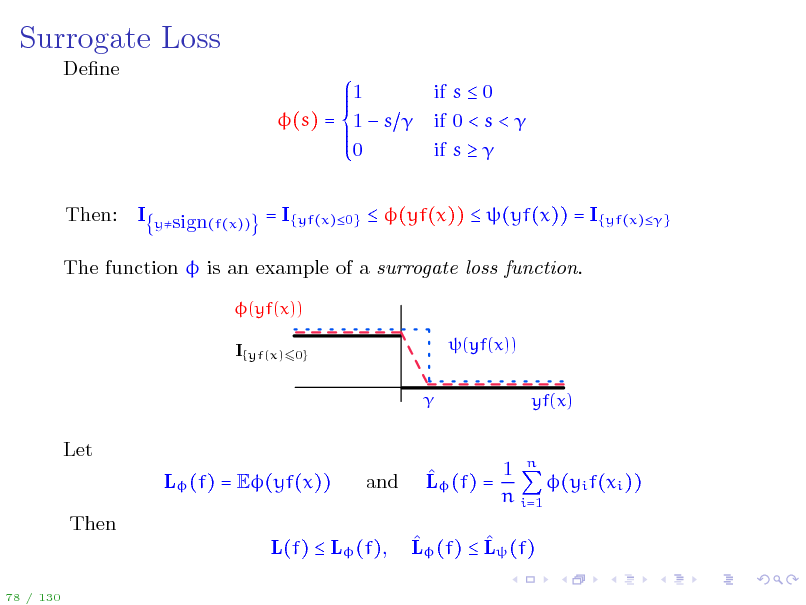
Surrogate Loss
Dene 1 (s) = 1 s 0 Then: I if s 0 if 0 < s < if s

ysign(f(x))

= I{yf(x)0} (yf(x)) (yf(x)) = I{yf(x)}

The function is an example of a surrogate loss function.
(yf(x)) I{yf(x)60} (yf(x)) yf(x)

Let L (f) = E(yf(x)) Then L(f) L (f),
78 / 130

and

1 n L (f) = (yi f(xi )) n i=1 L (f) L (f)

Surrogate Loss
Now consider uniform deviations for the surrogate loss: E sup L (f) L (f)
fF

We had shown that this quantity is at most 2Rn ((F)) for (F) = g(z) = (yf(x)) f F

A useful property of Rademacher averages: Rn ((F)) LRn (F) if is L-Lipschitz.

Observe that in our example is 1 -Lipschitz. Hence, 2 E sup L (f) L (f) Rn (F) fF

79 / 130

Margin Bound
Same result in high probability: with probability at least 1 , 2 sup L (f) L (f) Rn (F) + fF With probability at least 1 , for all f F 2 L(f) L (f) + Rn (F) + If fn is minimizing margin loss 1 n fn = arg min (yi f(xi )) fF n i=1 then with probability at least 1 L(fn ) inf L (f) +
fF

log(1 ) 2n

log(1 ) 2n

4 Rn (F) + 2

log(1 ) 2n

Note: assumes knowledge of , but this assumption can be removed.
80 / 130

Outline
Introduction Statistical Learning Theory The Setting of SLT Consistency, No Free Lunch Theorems, Bias-Variance Tradeo Tools from Probability, Empirical Processes From Finite to Innite Classes Uniform Convergence, Symmetrization, and Rademacher Complexity Large Margin Theory for Classication Properties of Rademacher Complexity Covering Numbers and Scale-Sensitive Dimensions Faster Rates Model Selection Sequential Prediction / Online Learning Motivation Supervised Learning Online Convex and Linear Optimization Online-to-Batch Conversion, SVM optimization

81 / 130

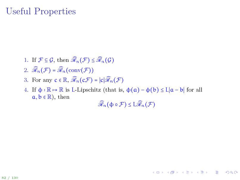
Useful Properties

1. If F G, then Rn (F) Rn (G) 2. Rn (F) = Rn (conv(F)) 3. For any c R, Rn (cF) = c Rn (F) 4. If R R is L-Lipschitz (that is, (a) (b) L a b for all a, b R), then Rn ( F) LRn (F)

82 / 130

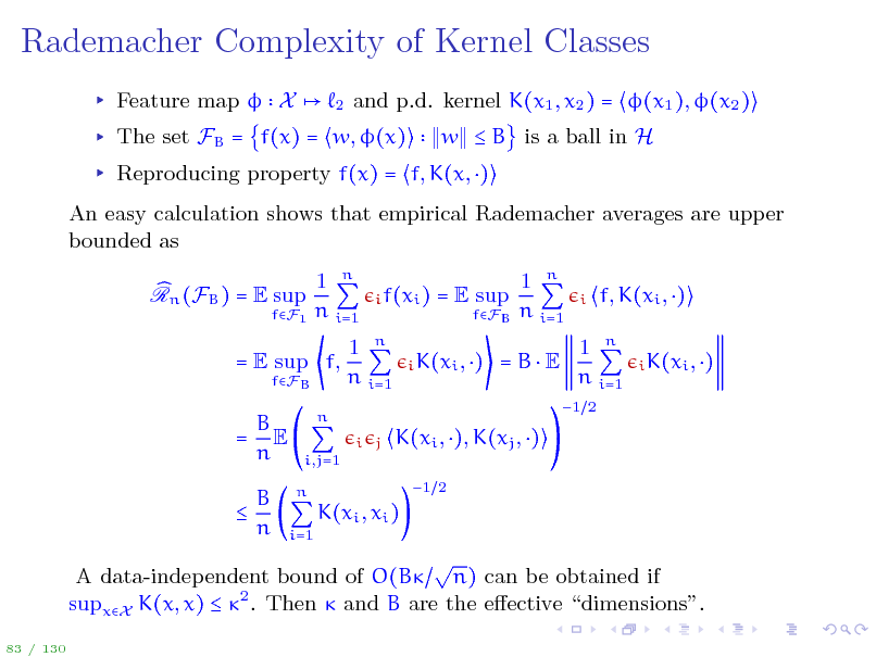
Rademacher Complexity of Kernel Classes
Feature map X
2

and p.d. kernel K(x1 , x2 ) = (x1 ), (x2 ) w B is a ball in H

The set FB = f(x) = w, (x)

Reproducing property f(x) = f, K(x, ) An easy calculation shows that empirical Rademacher averages are upper bounded as Rn (FB ) = E sup 1 n n i=1
i f(xi )

fF1

= E sup

fFB

1 n n i=1

i

f, K(xi , )
i K(xi , )

= E sup f,
fFB

1 n n i=1
i j

i K(xi , )

=BE

1 n n i=1
1 2

B = E n B n

n i,j=1 n i=1

K(xi , ), K(xj , )
1 2

K(xi , xi )

A data-independent bound of O(B n) can be obtained if supxX K(x, x) 2 . Then and B are the eective dimensions.
83 / 130

Other Examples

Using properties of Rademacher averages, we may establish guarantees for learning with neural networks, decision trees, and so on. Powerful technique, typically requires only a few lines of algebra. Occasionally, covering numbers and scale-sensitive dimensions can be easier to deal with.

84 / 130

Outline
Introduction Statistical Learning Theory The Setting of SLT Consistency, No Free Lunch Theorems, Bias-Variance Tradeo Tools from Probability, Empirical Processes From Finite to Innite Classes Uniform Convergence, Symmetrization, and Rademacher Complexity Large Margin Theory for Classication Properties of Rademacher Complexity Covering Numbers and Scale-Sensitive Dimensions Faster Rates Model Selection Sequential Prediction / Online Learning Motivation Supervised Learning Online Convex and Linear Optimization Online-to-Batch Conversion, SVM optimization

85 / 130

Real-Valued Functions: Covering Numbers
Consider a class F of [1, 1]-valued functions let Y = [1, 1], (f(x), y) = f(x) y We have E sup L(f) L(f) 2Ex1 n Rn (F)
fF

For real-valued functions the cardinality of F similar functions f and f with

x1 n

is innite. However,

(f(x1 ), . . . , f(xn )) (f (x1 ), . . . , f (xn )) should be treated as the same.

86 / 130

Real-Valued Functions: Covering Numbers
Given > 0, suppose we can nd V [1, 1]n of nite cardinality such that f, vf V, s.t. Then Rn (F) = E =E
1n

1 n f(xi ) vf i n i=1

sup
fF

1 n n i=1 1 n n i=1 max
vV

i f(xi ) i (f(xi )

1n

sup
fF

vf ) + E i

1n

sup
fF

1 n n i=1

f i vi

+E

1n

1 n n i=1

i vi

Now we are back to the set of nite cardinality: Rn (F) + 2 log card(V) n

87 / 130

Real-Valued Functions: Covering Numbers
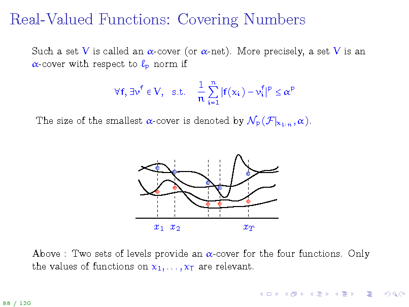
Such a set V is called an -cover (or -net). More precisely, a set V is an -cover with respect to p norm if f, vf V, s.t. 1 n f(xi ) vf p p i n i=1
x1 n , ).

The size of the smallest -cover is denoted by Np (F

x1 x2

xT

Above : Two sets of levels provide an -cover for the four functions. Only the values of functions on x1 , . . . , xT are relevant.

88 / 130

Real-Valued Functions: Covering Numbers

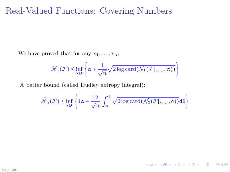
We have proved that for any x1 , . . . , xn , 1 Rn (F) inf + 0 n 2 log card(N1 (F
x1 n , ))

A better bound (called Dudley entropy integral): 12 Rn (F) inf 4 + 0 n
1

2 log card(N2 (F

x1 n , ))d

89 / 130

Example: Nondecreasing functions.
Consider the set F of nondecreasing functions R While F is a very large set, F N1 (F
x1 n

[1, 1].

is not that large:
x1 n , )

x1 n , )

N2 (F

n2 .

The rst bound on the previous slide yields 1 inf + n 4 log(n) = O(n1 3 )

0

while the second bound (the Dudley entropy integral) 12 inf 4 + 0 n
1

4 log(n)d = O(n1 2 )

where the O notation hides logarithmic factors.

90 / 130

Scale-Sensitive Dimensions
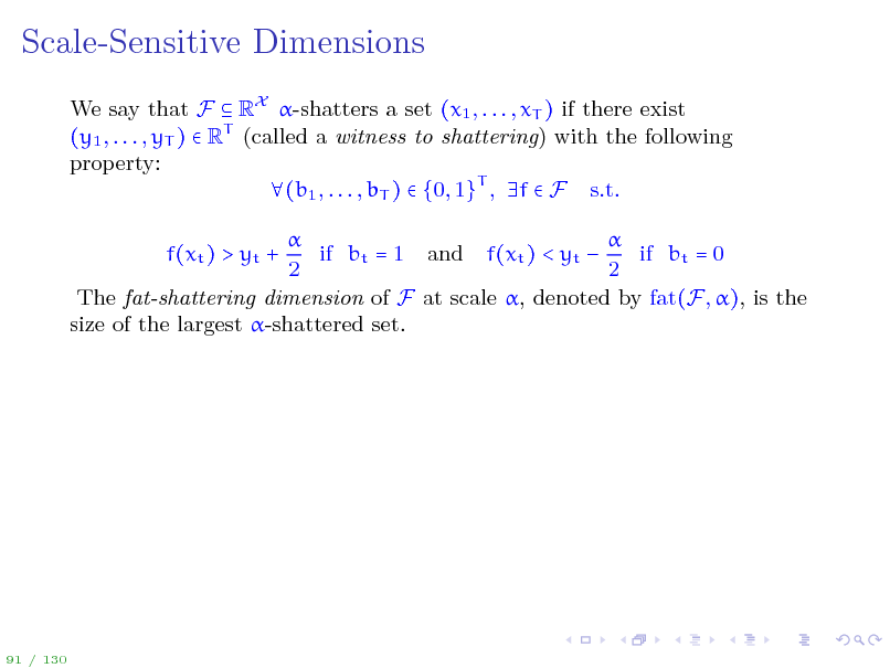
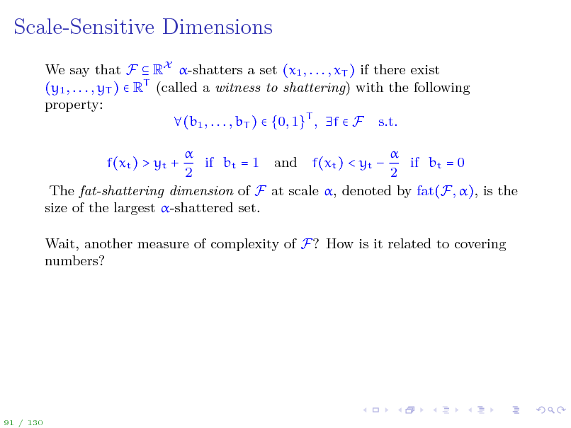
We say that F RX -shatters a set (x1 , . . . , xT ) if there exist (y1 , . . . , yT ) RT (called a witness to shattering) with the following property: (b1 , . . . , bT ) {0, 1}T , f F s.t. if bt = 1 and f(xt ) < yt if bt = 0 2 2 The fat-shattering dimension of F at scale , denoted by fat(F, ), is the size of the largest -shattered set. f(xt ) > yt +

91 / 130

Scale-Sensitive Dimensions
We say that F RX -shatters a set (x1 , . . . , xT ) if there exist (y1 , . . . , yT ) RT (called a witness to shattering) with the following property: (b1 , . . . , bT ) {0, 1}T , f F s.t. if bt = 1 and f(xt ) < yt if bt = 0 2 2 The fat-shattering dimension of F at scale , denoted by fat(F, ), is the size of the largest -shattered set. f(xt ) > yt + Wait, another measure of complexity of F? How is it related to covering numbers?

91 / 130

Scale-Sensitive Dimensions
We say that F RX -shatters a set (x1 , . . . , xT ) if there exist (y1 , . . . , yT ) RT (called a witness to shattering) with the following property: (b1 , . . . , bT ) {0, 1}T , f F s.t. if bt = 1 and f(xt ) < yt if bt = 0 2 2 The fat-shattering dimension of F at scale , denoted by fat(F, ), is the size of the largest -shattered set. f(xt ) > yt + Wait, another measure of complexity of F? How is it related to covering numbers? Theorem (Mendelson & Vershynin): For F [1, 1]X and any 0 < < 1, N2 (F
x1 n , )

2

Kfat(F ,c)

where K, c are positive absolute constants.

91 / 130

Quick Summary

We are after uniform deviations in order to understand performance of ERM. Rademacher averages is a nice measure with useful properties. They can be further upper bounded by covering numbers through the Dudley entropy integral. In turn, covering numbers can be controlled via the fat-shattering combinatorial dimension. Whew!

92 / 130

Outline
Introduction Statistical Learning Theory The Setting of SLT Consistency, No Free Lunch Theorems, Bias-Variance Tradeo Tools from Probability, Empirical Processes From Finite to Innite Classes Uniform Convergence, Symmetrization, and Rademacher Complexity Large Margin Theory for Classication Properties of Rademacher Complexity Covering Numbers and Scale-Sensitive Dimensions Faster Rates Model Selection Sequential Prediction / Online Learning Motivation Supervised Learning Online Convex and Linear Optimization Online-to-Batch Conversion, SVM optimization

93 / 130

Faster Rates

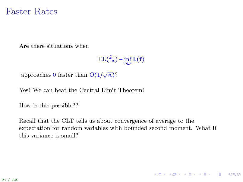
Are there situations when EL(fn ) inf L(f)
fF

approaches 0 faster than O(1

n)?

Yes! We can beat the Central Limit Theorem! How is this possible?? Recall that the CLT tells us about convergence of average to the expectation for random variables with bounded second moment. What if this variance is small?

94 / 130

Faster Rates: Classication
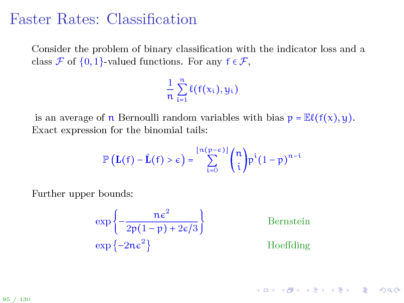
Consider the problem of binary classication with the indicator loss and a class F of {0, 1}-valued functions. For any f F, 1 n (f(xi ), yi ) n i=1 is an average of n Bernoulli random variables with bias p = E (f(x), y). Exact expression for the binomial tails: P L(f) L(f) > Further upper bounds: exp n 2 2p(1 p) + 2 3
2

=

n(p ) i=0

n i p (1 p)ni i

Bernstein Hoeding

exp 2n

95 / 130

Faster Rates: Classication
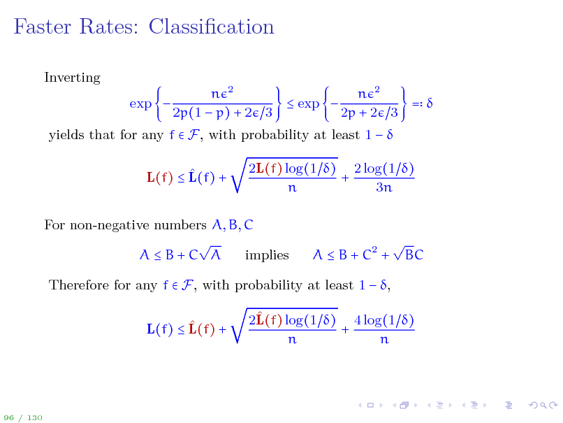
Inverting exp n 2 n 2 exp = 2p(1 p) + 2 3 2p + 2 3

yields that for any f F, with probability at least 1 L(f) L(f) + 2L(f) log(1 ) 2 log(1 ) + n 3n

For non-negative numbers A, B, C AB+C A implies

A B + C2 +

BC

Therefore for any f F, with probability at least 1 , L(f) L(f) + 2L(f) log(1 ) 4 log(1 ) + n n

96 / 130

Faster Rates: Classication
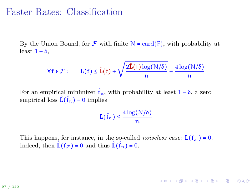
By the Union Bound, for F with nite N = card(F), with probability at least 1 , f F L(f) L(f) + 2L(f) log(N ) 4 log(N ) + n n

For an empirical minimizer fn , with probability at least 1 , a zero empirical loss L(fn ) = 0 implies L(fn ) 4 log(N ) n

This happens, for instance, in the so-called noiseless case: L(fF ) = 0. Indeed, then L(fF ) = 0 and thus L(fn ) = 0.

97 / 130

Summary: Minimax Viewpoint

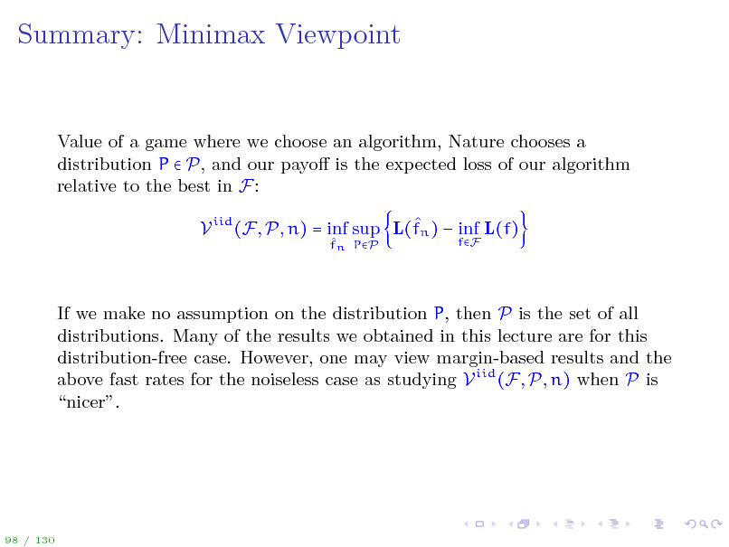
Value of a game where we choose an algorithm, Nature chooses a distribution P P, and our payo is the expected loss of our algorithm relative to the best in F: V iid (F, P, n) = inf sup L(fn ) inf L(f)
fn PP fF

If we make no assumption on the distribution P, then P is the set of all distributions. Many of the results we obtained in this lecture are for this distribution-free case. However, one may view margin-based results and the above fast rates for the noiseless case as studying V iid (F, P, n) when P is nicer.

98 / 130

Outline
Introduction Statistical Learning Theory The Setting of SLT Consistency, No Free Lunch Theorems, Bias-Variance Tradeo Tools from Probability, Empirical Processes From Finite to Innite Classes Uniform Convergence, Symmetrization, and Rademacher Complexity Large Margin Theory for Classication Properties of Rademacher Complexity Covering Numbers and Scale-Sensitive Dimensions Faster Rates Model Selection Sequential Prediction / Online Learning Motivation Supervised Learning Online Convex and Linear Optimization Online-to-Batch Conversion, SVM optimization

99 / 130

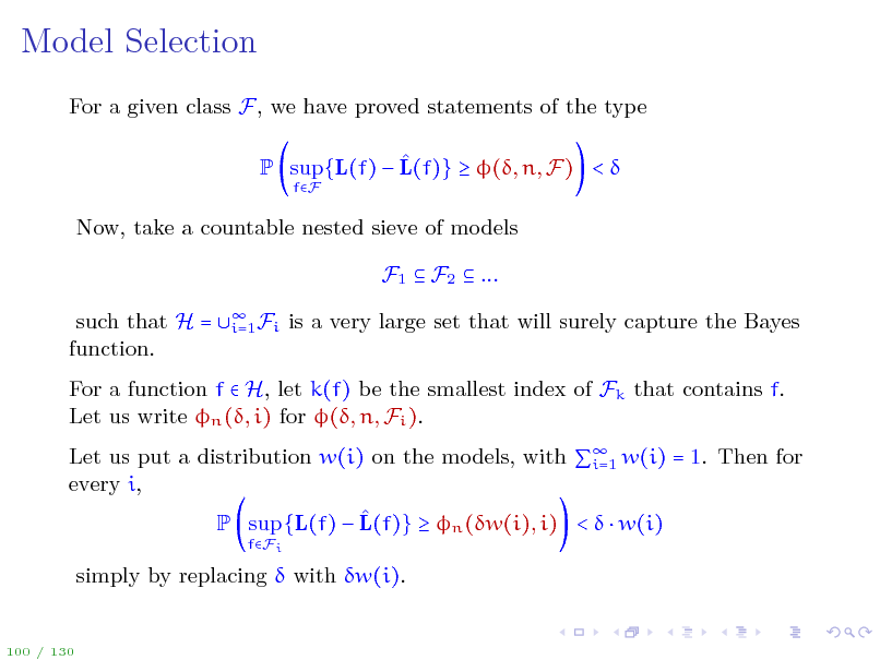
Model Selection
For a given class F, we have proved statements of the type P sup{L(f) L(f)} (, n, F) <
fF

Now, take a countable nested sieve of models F1 F2 ... such that H = function. Fi i=1 is a very large set that will surely capture the Bayes

For a function f H, let k(f) be the smallest index of Fk that contains f. Let us write n (, i) for (, n, Fi ). Let us put a distribution w(i) on the models, with w(i) = 1. Then for i=1 every i, P sup {L(f) L(f)} n (w(i), i) < w(i)
fFi

simply by replacing with w(i).

100 / 130

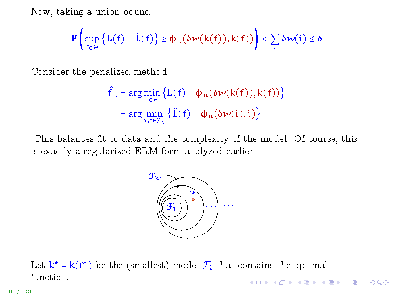
Now, taking a union bound: P sup L(f) L(f) n (w(k(f)), k(f)) <
fH i

w(i)

Consider the penalized method fn = arg min L(f) + n (w(k(f)), k(f))
fH

= arg min L(f) + n (w(i), i)
i,fFi

This balances t to data and the complexity of the model. Of course, this is exactly a regularized ERM form analyzed earlier.
F k f F1 ... ...

Let k = k(f ) be the (smallest) model Fi that contains the optimal function.
101 / 130

Exactly as on the slide Countable Class: Weighted Union Bound, L(fn ) L(f ) L(fn ) L(fn ) penn (fn ) + L(fn ) + penn (fn ) L(fF ) penn (fF ) + L(fF ) L(fF ) + penn (fF ) L(f ) L(f ) + penn (f ) = L(f ) L(f ) + n (w(k ), k ) The rst part of this bound is OP (1 n) by the CLT, just as before. If the dependence of on 1 is logarithmic, then taking w(i) = 2i simply implies an additional additive i , a penalty for not knowing the model in advance. Conclusion: given uniform deviation bounds for a single class F, as developed earlier, we can perform model selection by penalizing model complexity!

102 / 130

Outline
Introduction Statistical Learning Theory The Setting of SLT Consistency, No Free Lunch Theorems, Bias-Variance Tradeo Tools from Probability, Empirical Processes From Finite to Innite Classes Uniform Convergence, Symmetrization, and Rademacher Complexity Large Margin Theory for Classication Properties of Rademacher Complexity Covering Numbers and Scale-Sensitive Dimensions Faster Rates Model Selection Sequential Prediction / Online Learning Motivation Supervised Learning Online Convex and Linear Optimization Online-to-Batch Conversion, SVM optimization

103 / 130

Outline
Introduction Statistical Learning Theory The Setting of SLT Consistency, No Free Lunch Theorems, Bias-Variance Tradeo Tools from Probability, Empirical Processes From Finite to Innite Classes Uniform Convergence, Symmetrization, and Rademacher Complexity Large Margin Theory for Classication Properties of Rademacher Complexity Covering Numbers and Scale-Sensitive Dimensions Faster Rates Model Selection Sequential Prediction / Online Learning Motivation Supervised Learning Online Convex and Linear Optimization Online-to-Batch Conversion, SVM optimization

104 / 130

Looking back: Statistical Learning

future looks like the past modeled as i.i.d. data evaluated on a random sample from the same distribution developed various measures of complexity of F

105 / 130

Example #1: Bit Prediction

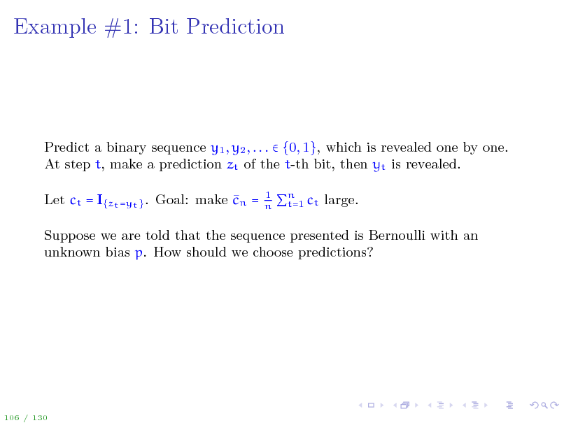
Predict a binary sequence y1 , y2 , . . . {0, 1}, which is revealed one by one. At step t, make a prediction zt of the t-th bit, then yt is revealed. Let ct = I{zt =yt } . Goal: make cn =
1 n n t=1 ct large.

Suppose we are told that the sequence presented is Bernoulli with an unknown bias p. How should we choose predictions?

106 / 130

Example #1: Bit Prediction
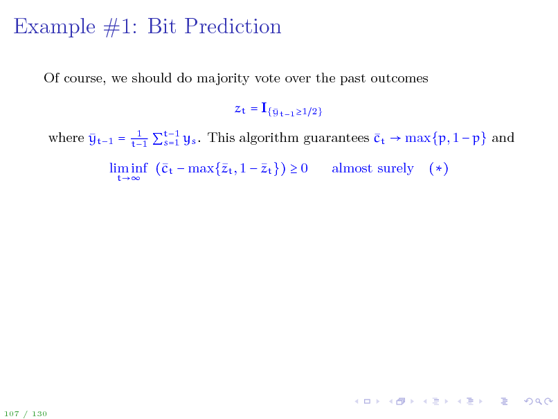
Of course, we should do majority vote over the past outcomes zt = I{ t1 1 y where yt1 =
1 t1 2}

t1 s=1 ys . This algorithm guarantees ct max{p, 1 p} and

lim inf (t max{t , 1 zt }) 0 c z
t

almost surely

()

107 / 130

Example #1: Bit Prediction
Of course, we should do majority vote over the past outcomes zt = I{ t1 1 y where yt1 =
1 t1 2}

t1 s=1 ys . This algorithm guarantees ct max{p, 1 p} and

lim inf (t max{t , 1 zt }) 0 c z
t

almost surely

()

Claim: there is an algorithm that ensures () for an arbitrary sequence. Any idea how to do it?

107 / 130

Example #1: Bit Prediction
Of course, we should do majority vote over the past outcomes zt = I{ t1 1 y where yt1 =
1 t1 2}

t1 s=1 ys . This algorithm guarantees ct max{p, 1 p} and

lim inf (t max{t , 1 zt }) 0 c z
t

almost surely

()

Claim: there is an algorithm that ensures () for an arbitrary sequence. Any idea how to do it? Another way to formulate (): number of mistakes should be not much more than made by the best of the two experts, one predicting 1 all the time, the other constantly predicting 0.

107 / 130

Example #1: Bit Prediction
Of course, we should do majority vote over the past outcomes zt = I{ t1 1 y where yt1 =
1 t1 2}

t1 s=1 ys . This algorithm guarantees ct max{p, 1 p} and

lim inf (t max{t , 1 zt }) 0 c z
t

almost surely

()

Claim: there is an algorithm that ensures () for an arbitrary sequence. Any idea how to do it? Another way to formulate (): number of mistakes should be not much more than made by the best of the two experts, one predicting 1 all the time, the other constantly predicting 0. Note the dierence: estimating a hypothesized model vs competing against a reference set. We had seen this distinction in the previous lecture.

107 / 130

Example #2: Email Spam Detection

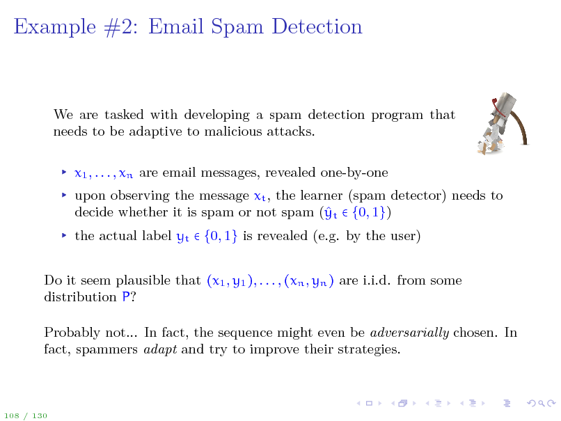
We are tasked with developing a spam detection program that needs to be adaptive to malicious attacks. x1 , . . . , xn are email messages, revealed one-by-one upon observing the message xt , the learner (spam detector) needs to decide whether it is spam or not spam ( t {0, 1}) y the actual label yt {0, 1} is revealed (e.g. by the user) Do it seem plausible that (x1 , y1 ), . . . , (xn , yn ) are i.i.d. from some distribution P? Probably not... In fact, the sequence might even be adversarially chosen. In fact, spammers adapt and try to improve their strategies.

108 / 130

Outline
Introduction Statistical Learning Theory The Setting of SLT Consistency, No Free Lunch Theorems, Bias-Variance Tradeo Tools from Probability, Empirical Processes From Finite to Innite Classes Uniform Convergence, Symmetrization, and Rademacher Complexity Large Margin Theory for Classication Properties of Rademacher Complexity Covering Numbers and Scale-Sensitive Dimensions Faster Rates Model Selection Sequential Prediction / Online Learning Motivation Supervised Learning Online Convex and Linear Optimization Online-to-Batch Conversion, SVM optimization

109 / 130

Online Learning (Supervised)
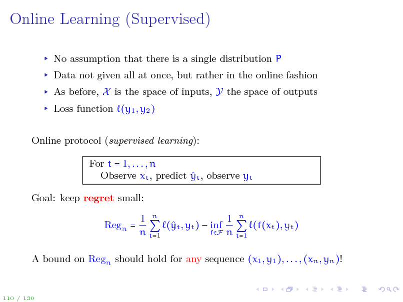
No assumption that there is a single distribution P Data not given all at once, but rather in the online fashion As before, X is the space of inputs, Y the space of outputs Loss function (y1 , y2 ) Online protocol (supervised learning): For t = 1, . . . , n Observe xt , predict yt , observe yt Goal: keep regret small: Regn = 1 n 1 n ( t , yt ) inf y (f(xt ), yt ) fF n t=1 n t=1

A bound on Regn should hold for any sequence (x1 , y1 ), . . . , (xn , yn )!

110 / 130

Pros/Cons of Online Learning
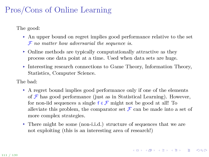
The good: An upper bound on regret implies good performance relative to the set F no matter how adversarial the sequence is. Online methods are typically computationally attractive as they process one data point at a time. Used when data sets are huge. Interesting research connections to Game Theory, Information Theory, Statistics, Computer Science. The bad: A regret bound implies good performance only if one of the elements of F has good performance (just as in Statistical Learning). However, for non-iid sequences a single f F might not be good at all! To alleviate this problem, the comparator set F can be made into a set of more complex strategies. There might be some (non-i.i.d.) structure of sequences that we are not exploiting (this is an interesting area of research!)

111 / 130

Setting Up the Minimax Value
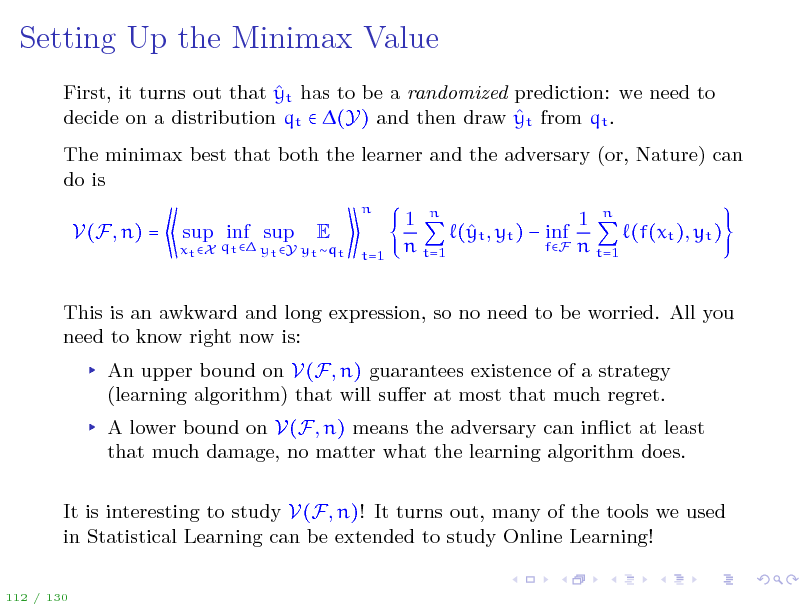
First, it turns out that yt has to be a randomized prediction: we need to decide on a distribution qt (Y) and then draw yt from qt . The minimax best that both the learner and the adversary (or, Nature) can do is
n

V(F, n) =

xt X qt yt Y yt qt

sup inf sup

E

t=1

1 n 1 n ( t , yt ) inf y (f(xt ), yt ) fF n t=1 n t=1

This is an awkward and long expression, so no need to be worried. All you need to know right now is: An upper bound on V(F, n) guarantees existence of a strategy (learning algorithm) that will suer at most that much regret. A lower bound on V(F, n) means the adversary can inict at least that much damage, no matter what the learning algorithm does. It is interesting to study V(F, n)! It turns out, many of the tools we used in Statistical Learning can be extended to study Online Learning!
112 / 130

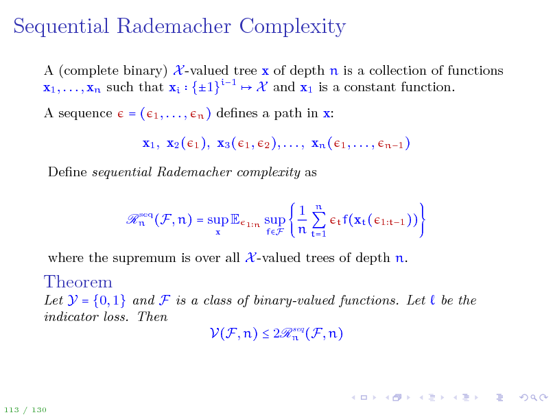
Sequential Rademacher Complexity
A (complete binary) X -valued tree x of depth n is a collection of functions x1 , . . . , xn such that xi {1}i1 X and x1 is a constant function. A sequence =(
1, . . . , n) 1 ),

denes a path in x: x3 (
1, 2 ), . . . ,

x1 , x2 (

xn (

1, . . . ,

n1 )

Dene sequential Rademacher complexity as
seq Rn (F, n) = sup E

x

1n

sup
fF

1 n n t=1

t f(xt ( 1 t1 ))

where the supremum is over all X -valued trees of depth n.

Theorem

Let Y = {0, 1} and F is a class of binary-valued functions. Let indicator loss. Then seq V(F, n) 2Rn (F, n)

be the

113 / 130

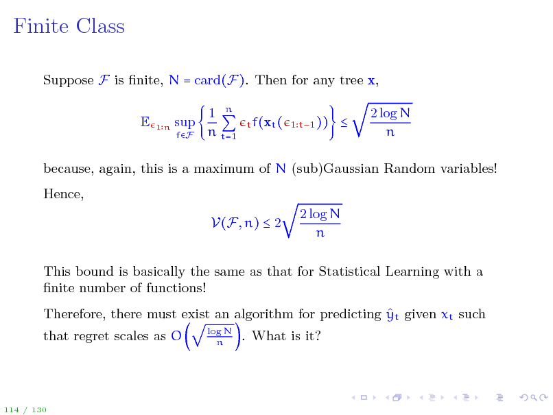
Finite Class
Suppose F is nite, N = card(F). Then for any tree x, E
1n

sup
fF

1 n n t=1

t f(xt ( 1 t1 ))

2 log N n

because, again, this is a maximum of N (sub)Gaussian Random variables! Hence, V(F, n) 2 2 log N n

This bound is basically the same as that for Statistical Learning with a nite number of functions! Therefore, there must exist an algorithm for predicting yt given xt such that regret scales as O
log N n

. What is it?

114 / 130

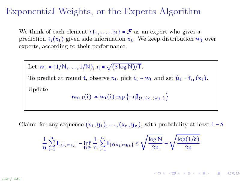
Exponential Weights, or the Experts Algorithm
We think of each element {f1 , . . . , fN } = F as an expert who gives a prediction fi (xt ) given side information xt . We keep distribution wt over experts, according to their performance. Let w1 = (1 N, . . . , 1 N), = (8 log N) T .

To predict at round t, observe xt , pick it wt and set yt = fit (xt ). Update wt+1 (i) wt (i) exp I{fi (xt )yt }

Claim: for any sequence (x1 , y1 ), . . . , (xn , yn ), with probability at least 1 1 n 1 n I{ t yt } inf I{f(xt )yt } y fF n t=1 n t=1 log N + 2n log(1 ) 2n

115 / 130

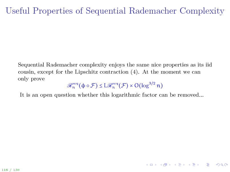
Useful Properties of Sequential Rademacher Complexity

Sequential Rademacher complexity enjoys the same nice properties as its iid cousin, except for the Lipschitz contraction (4). At the moment we can only prove seq seq Rn ( F) LRn (F) O(log3 2 n) It is an open question whether this logarithmic factor can be removed...

116 / 130

Theory for Online Learning

There is now a theory with combinatorial parameters, covering numbers, and even a recipe for developing online algorithms! Many of the relevant concepts (e.g. sequential Rademacher complexity) are generalizations of the i.i.d. analogues to the case of dependent data. Coupled with the online-to-batch conversion we introduce in a few slides, there is now an interesting possibility of developing new computationally attractive algorithms for statistical learning. One such example will be presented.

117 / 130

Theory for Online Learning

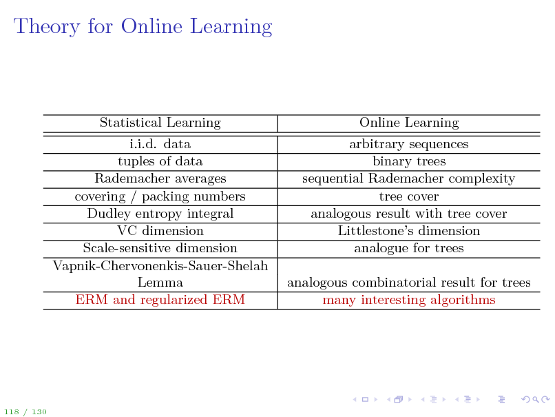
Statistical Learning i.i.d. data tuples of data Rademacher averages covering / packing numbers Dudley entropy integral VC dimension Scale-sensitive dimension Vapnik-Chervonenkis-Sauer-Shelah Lemma ERM and regularized ERM

Online Learning arbitrary sequences binary trees sequential Rademacher complexity tree cover analogous result with tree cover Littlestones dimension analogue for trees analogous combinatorial result for trees many interesting algorithms

118 / 130

Outline
Introduction Statistical Learning Theory The Setting of SLT Consistency, No Free Lunch Theorems, Bias-Variance Tradeo Tools from Probability, Empirical Processes From Finite to Innite Classes Uniform Convergence, Symmetrization, and Rademacher Complexity Large Margin Theory for Classication Properties of Rademacher Complexity Covering Numbers and Scale-Sensitive Dimensions Faster Rates Model Selection Sequential Prediction / Online Learning Motivation Supervised Learning Online Convex and Linear Optimization Online-to-Batch Conversion, SVM optimization

119 / 130

Online Convex and Linear Optimization

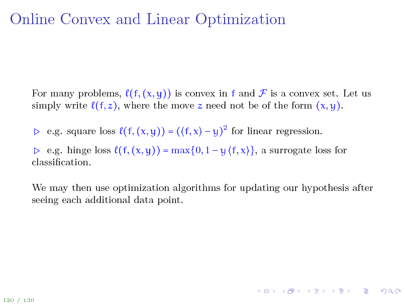
For many problems, (f, (x, y)) is convex in f and F is a convex set. Let us simply write (f, z), where the move z need not be of the form (x, y). e.g. square loss (f, (x, y)) = ( f, x y)2 for linear regression. e.g. hinge loss (f, (x, y)) = max{0, 1 y f, x }, a surrogate loss for classication. We may then use optimization algorithms for updating our hypothesis after seeing each additional data point.

120 / 130

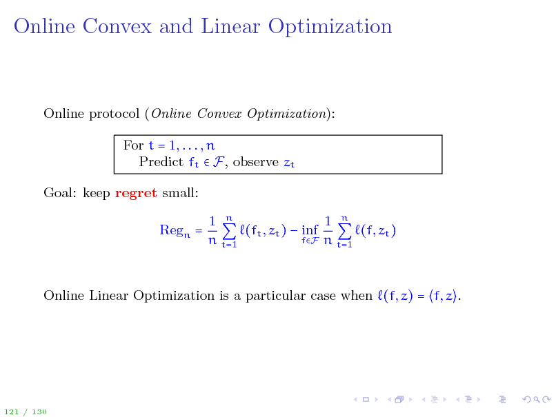
Online Convex and Linear Optimization

Online protocol (Online Convex Optimization): For t = 1, . . . , n Predict ft F, observe zt Goal: keep regret small: Regn = 1 n 1 n (ft , zt ) inf (f, zt ) fF n t=1 n t=1

Online Linear Optimization is a particular case when (f, z) = f, z .

121 / 130

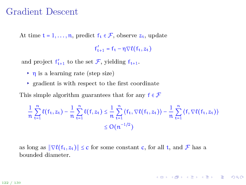
Gradient Descent
At time t = 1, . . . , n, predict ft F, observe zt , update
ft+1 = ft (ft , zt ) and project ft+1 to the set F, yielding ft+1 .

is a learning rate (step size) gradient is with respect to the rst coordinate This simple algorithm guarantees that for any f F 1 n 1 n 1 n 1 n (ft , zt ) (f, zt ) ft , (ft , zt ) f, (ft , zt ) n t=1 n t=1 n t=1 n t=1 O(n1 2 ) as long as (ft , zt ) c for some constant c, for all t, and F has a bounded diameter.

122 / 130

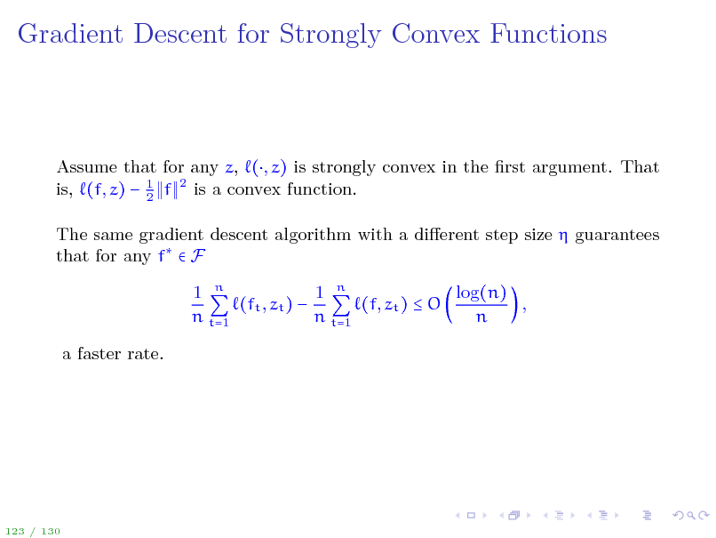
Gradient Descent for Strongly Convex Functions

Assume that for any z, (, z) is strongly convex in the rst argument. That is, (f, z) 1 f 2 is a convex function. 2 The same gradient descent algorithm with a dierent step size guarantees that for any f F log(n) 1 n 1 n (ft , zt ) (f, zt ) O , n t=1 n t=1 n a faster rate.

123 / 130

Outline
Introduction Statistical Learning Theory The Setting of SLT Consistency, No Free Lunch Theorems, Bias-Variance Tradeo Tools from Probability, Empirical Processes From Finite to Innite Classes Uniform Convergence, Symmetrization, and Rademacher Complexity Large Margin Theory for Classication Properties of Rademacher Complexity Covering Numbers and Scale-Sensitive Dimensions Faster Rates Model Selection Sequential Prediction / Online Learning Motivation Supervised Learning Online Convex and Linear Optimization Online-to-Batch Conversion, SVM optimization

124 / 130

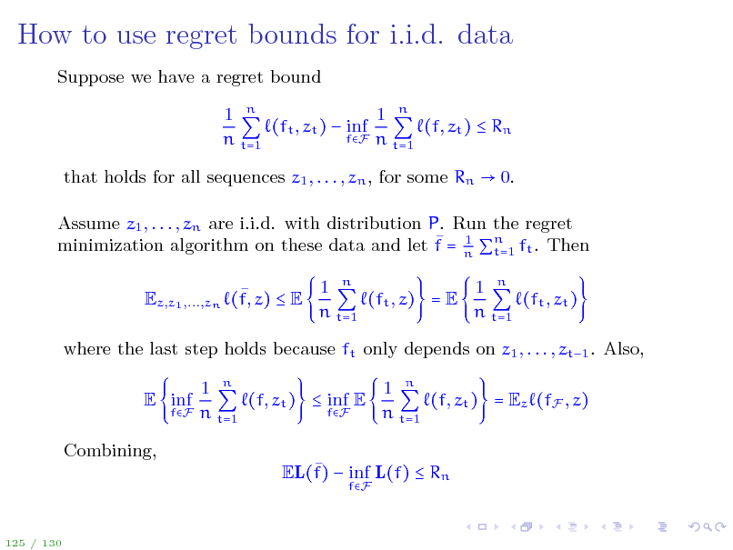
How to use regret bounds for i.i.d. data
Suppose we have a regret bound 1 n 1 n (ft , zt ) inf (f, zt ) Rn fF n t=1 n t=1 that holds for all sequences z1 , . . . , zn , for some Rn 0. Assume z1 , . . . , zn are i.i.d. with distribution P. Run the regret 1 t=1 minimization algorithm on these data and let f = n n ft . Then Ez,z1 ,...,zn (f, z) E 1 n 1 n (ft , z) = E (ft , zt ) n t=1 n t=1

where the last step holds because ft only depends on z1 , . . . , zt1 . Also, E inf Combining, EL(f) inf L(f) Rn
fF

fF

1 n 1 n (f, zt ) inf E (f, zt ) = Ez (fF , z) fF n t=1 n t=1

125 / 130

How to use regret bounds for i.i.d. data

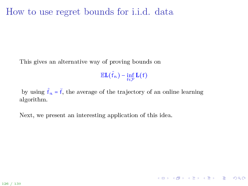
This gives an alternative way of proving bounds on EL(fn ) inf L(f)
fF

by using fn = f, the average of the trajectory of an online learning algorithm. Next, we present an interesting application of this idea.

126 / 130

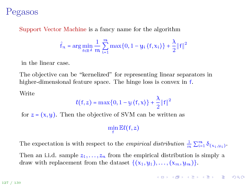
Pegasos
Support Vector Machine is a fancy name for the algorithm 1 m max{0, 1 yi f, xi } + f fn = arg min d m 2 fR i=1 in the linear case. The objective can be kernelized for representing linear separators in higher-dimensional feature space. The hinge loss is convex in f. Write 2 f 2 for z = (x, y). Then the objective of SVM can be written as (f, z) = max{0, 1 y f, x } + min E (f, z)
f 2

The expectation is with respect to the empirical distribution

1 m

i=1 (xi ,yi ) .

m

Then an i.i.d. sample z1 , . . . , zn from the empirical distribution is simply a draw with replacement from the dataset {(x1 , y1 ), . . . , (xm , ym )}.
127 / 130

Pegasos
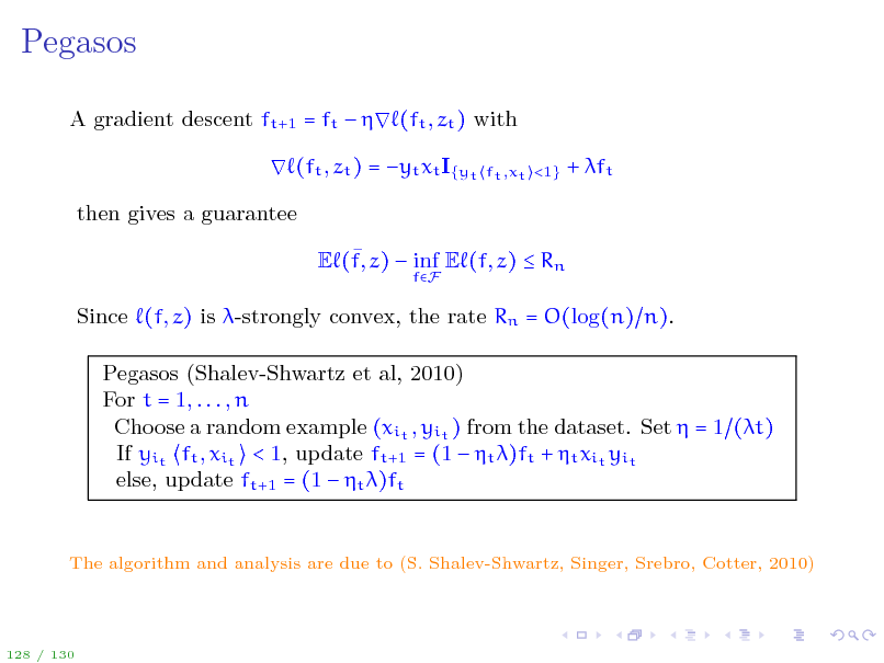
A gradient descent ft+1 = ft (ft , zt ) with (ft , zt ) = yt xt I{yt then gives a guarantee E (f, z) inf E (f, z) Rn
fF ft ,xt <1}

+ ft

Since (f, z) is -strongly convex, the rate Rn = O(log(n) n). Pegasos (Shalev-Shwartz et al, 2010) For t = 1, . . . , n Choose a random example (xit , yit ) from the dataset. Set = 1 (t) If yit ft , xit < 1, update ft+1 = (1 t )ft + t xit yit else, update ft+1 = (1 t )ft

The algorithm and analysis are due to (S. Shalev-Shwartz, Singer, Srebro, Cotter, 2010)

128 / 130

Pegasos

1 t=1 We conclude that f = n n ft computed using the gradient descent 1 )-approximate minimizer of the SVM objective after algorithm is an O(n n steps. This gives an O(d ( )) time to converge to an -minimizer. Very fast SVM solver, attractive for large datasets!

129 / 130

Summary

Key points for both statistical and online learning: obtained performance guarantees with minimal assumptions prior knowledge is captured by the comparator term understanding the inherent complexity of the comparator set key techniques: empirical processes for iid and non-iid data interesting relationships between statistical and online learning computation and statistics a basis of machine learning

130 / 130