
MLSS2012, Kyoto, Japan
Sep. 7, 2012
Density Ratio Estimation in Machine Learning
Masashi Sugiyama Tokyo Institute of Technology, Japan
sugi@cs.titech.ac.jp http://sugiyama-www.cs.titech.ac.jp/~sugi/
In statistical machine learning, avoiding density estimation is essential because it is often more difficult than solving a target machine learning problem itself. This is often referred to as Vapnik's principle, and the support vector machine is one of the successful realizations of this principle. Following this spirit, a new machine learning framework based on the ratio of probability density functions has been introduced. This density-ratio framework includes various important machine learning tasks such as transfer learning, outlier detection, feature selection, clustering, and conditional density estimation. All these tasks can be effectively and efficiently solved in a unified manner by estimating directly the density ratio without actually going through density estimation. In this lecture, I give an overview of theory, algorithms, and application of density ratio estimation.
Scroll with j/k | | | Size
MLSS2012, Kyoto, Japan
Sep. 7, 2012
Density Ratio Estimation in Machine Learning
Masashi Sugiyama Tokyo Institute of Technology, Japan
sugi@cs.titech.ac.jp http://sugiyama-www.cs.titech.ac.jp/~sugi/
1
Generative Approach to Machine Learning (ML)
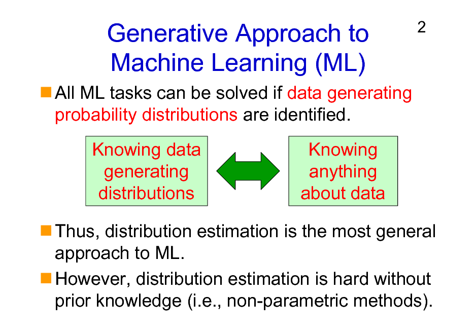
All ML tasks can be solved if data generating probability distributions are identified. Knowing data generating distributions Knowing anything about data
2
Thus, distribution estimation is the most general approach to ML. However, distribution estimation is hard without prior knowledge (i.e., non-parametric methods).
2
Discriminative Approach to ML
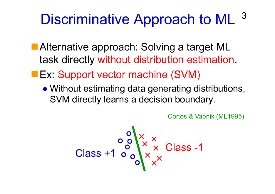
Alternative approach: Solving a target ML task directly without distribution estimation. Ex: Support vector machine (SVM)
3
Without estimating data generating distributions, SVM directly learns a decision boundary.
Cortes & Vapnik (ML1995)
Class +1
Class -1
3
Discriminative Approach to ML
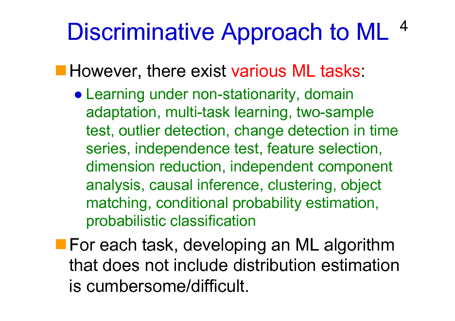
However, there exist various ML tasks:
Learning under non-stationarity, domain adaptation, multi-task learning, two-sample test, outlier detection, change detection in time series, independence test, feature selection, dimension reduction, independent component analysis, causal inference, clustering, object matching, conditional probability estimation, probabilistic classification
4
For each task, developing an ML algorithm that does not include distribution estimation is cumbersome/difficult.
4
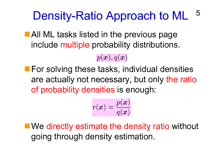
Density-Ratio Approach to ML
All ML tasks listed in the previous page include multiple probability distributions.
5
For solving these tasks, individual densities are actually not necessary, but only the ratio of probability densities is enough:
We directly estimate the density ratio without going through density estimation.
5
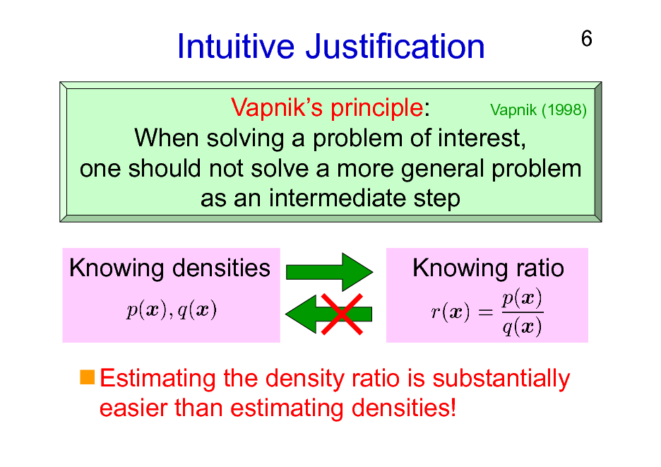
Intuitive Justification
6
Vapnik (1998) Vapniks principle: When solving a problem of interest, one should not solve a more general problem as an intermediate step
Knowing densities
Knowing ratio
Estimating the density ratio is substantially easier than estimating densities!
6
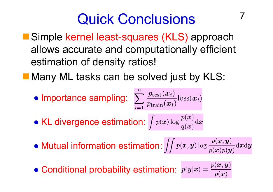
Quick Conclusions
Simple kernel least-squares (KLS) approach allows accurate and computationally efficient estimation of density ratios! Many ML tasks can be solved just by KLS:
Importance sampling: KL divergence estimation: Mutual information estimation: Conditional probability estimation:
7
7
Books on Density Ratios
Sugiyama, Suzuki & Kanamori, Density Ratio Estimation in Machine Learning, Cambridge University Press, 2012
8
Sugiyama & Kawanabe Machine Learning in Non-Stationary Environments, MIT Press, 2012
8
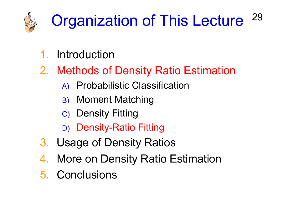
Organization of This Lecture
1. 2. 3. 4. 5. Introduction Methods of Density Ratio Estimation Usage of Density Ratios More on Density Ratio Estimation Conclusions
9
9
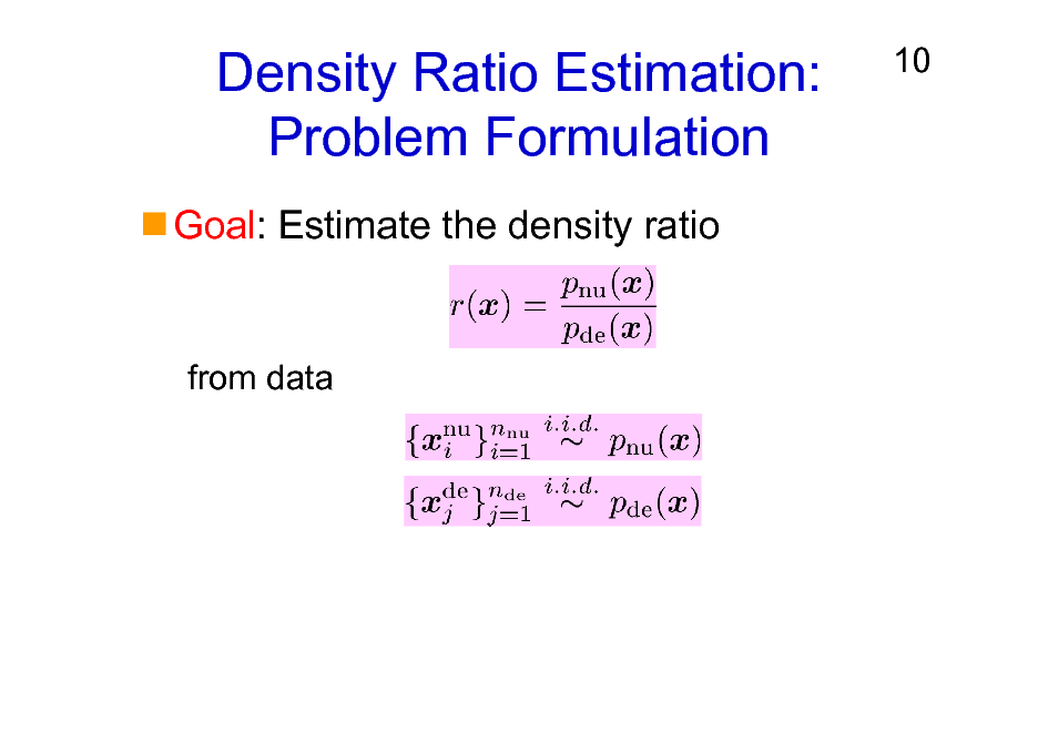
Density Ratio Estimation: Problem Formulation
Goal: Estimate the density ratio
10
from data
10
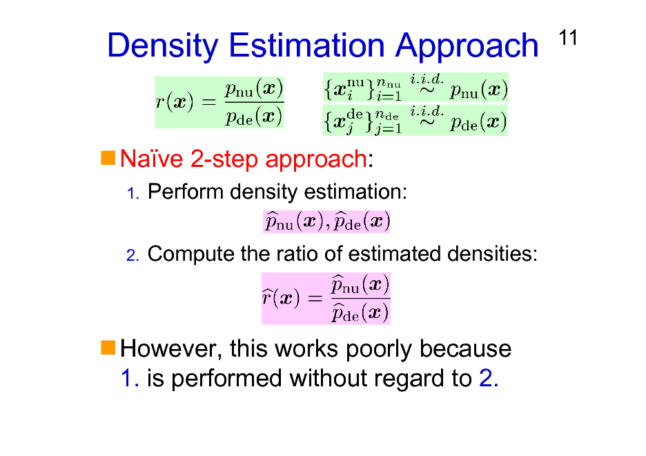
Density Estimation Approach
Nave 2-step approach:
1.
11
Perform density estimation: Compute the ratio of estimated densities:
2.
However, this works poorly because 1. is performed without regard to 2.
11
Organization of This Lecture
1. Introduction 2. Methods of Density Ratio Estimation
A) B) C) D)
12
Probabilistic Classification Moment Matching Density Fitting Density-Ratio Fitting
3. Usage of Density Ratios 4. More on Density Ratio Estimation 5. Conclusions
12
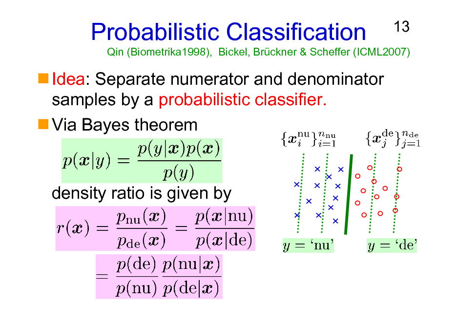
Probabilistic Classification
Idea: Separate numerator and denominator samples by a probabilistic classifier. Via Bayes theorem
13
Qin (Biometrika1998), Bickel, Brckner & Scheffer (ICML2007)
density ratio is given by
13
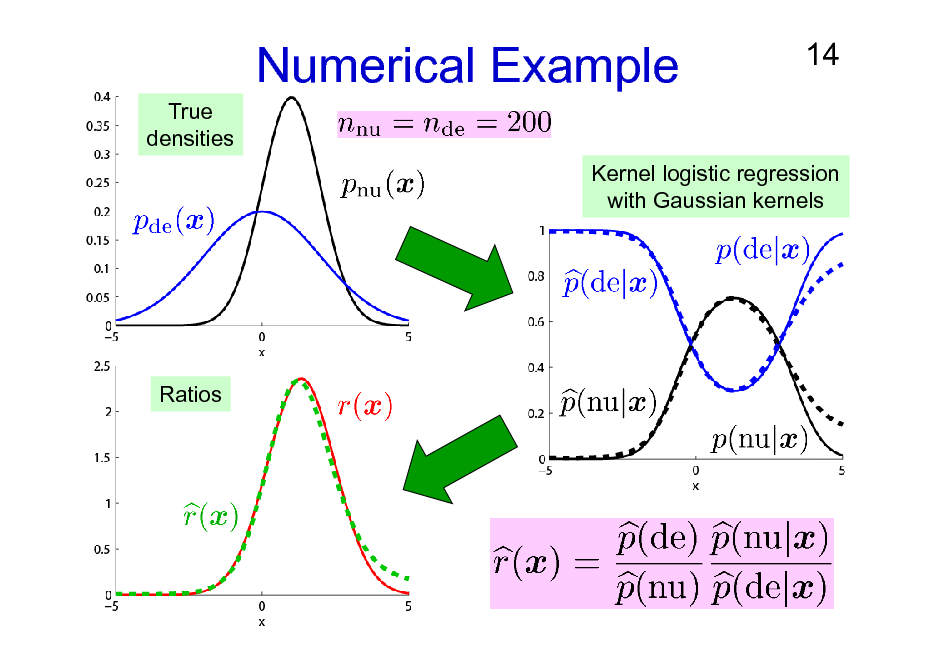
Numerical Example
True densities
14
Kernel logistic regression with Gaussian kernels
Ratios
14
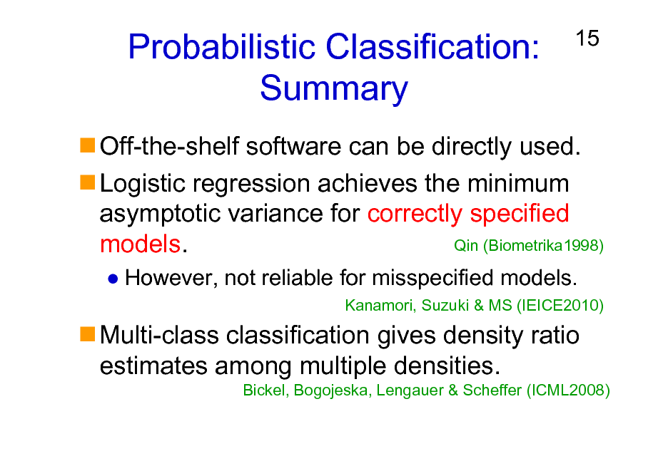
Probabilistic Classification: Summary
15
Off-the-shelf software can be directly used. Logistic regression achieves the minimum asymptotic variance for correctly specified Qin (Biometrika1998) models.
However, not reliable for misspecified models.
Kanamori, Suzuki & MS (IEICE2010)
Multi-class classification gives density ratio estimates among multiple densities.
Bickel, Bogojeska, Lengauer & Scheffer (ICML2008)
15
Organization of This Lecture
1. Introduction 2. Methods of Density Ratio Estimation
A) B) C) D)
16
Probabilistic Classification Moment Matching Density Fitting Density-Ratio Fitting
3. Usage of Density Ratios 4. More on Density Ratio Estimation 5. Conclusions
16
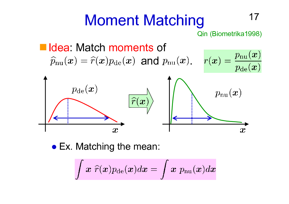
Moment Matching
Idea: Match moments of and .
17
Qin (Biometrika1998)
Ex. Matching the mean:
17
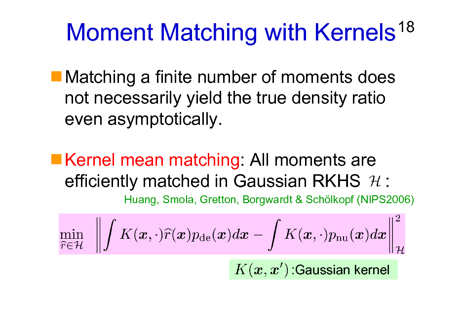
Moment Matching with Kernels
Matching a finite number of moments does not necessarily yield the true density ratio even asymptotically. Kernel mean matching: All moments are efficiently matched in Gaussian RKHS :
18
Huang, Smola, Gretton, Borgwardt & Schlkopf (NIPS2006)
:Gaussian kernel
18
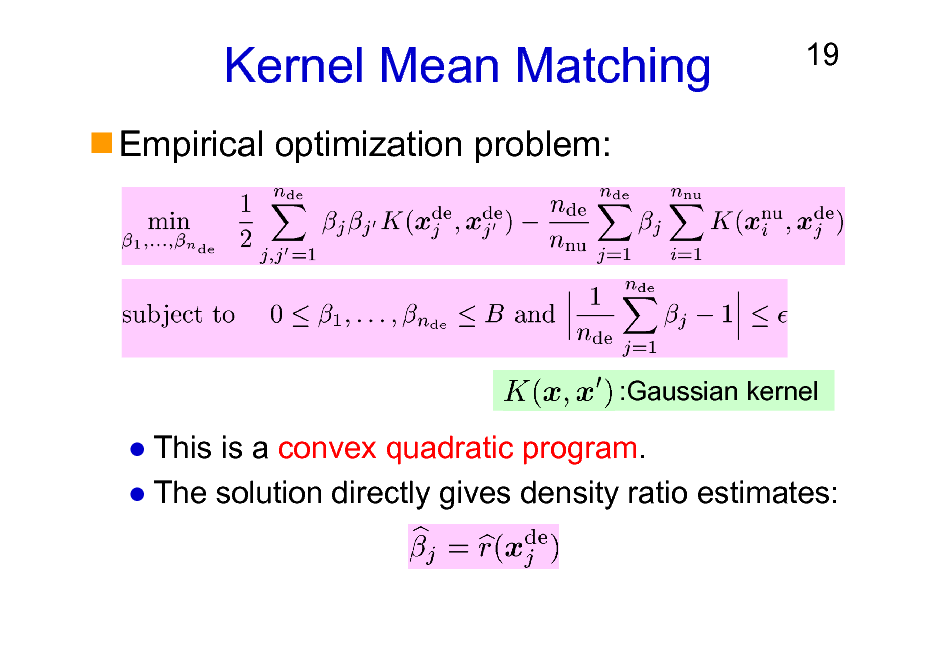
Kernel Mean Matching
Empirical optimization problem:
19
:Gaussian kernel
This is a convex quadratic program. The solution directly gives density ratio estimates:
19
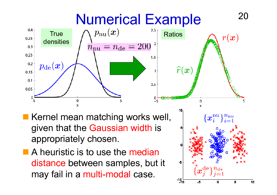
Numerical Example
True densities Ratios
20
Kernel mean matching works well, given that the Gaussian width is appropriately chosen. A heuristic is to use the median distance between samples, but it may fail in a multi-modal case.
20
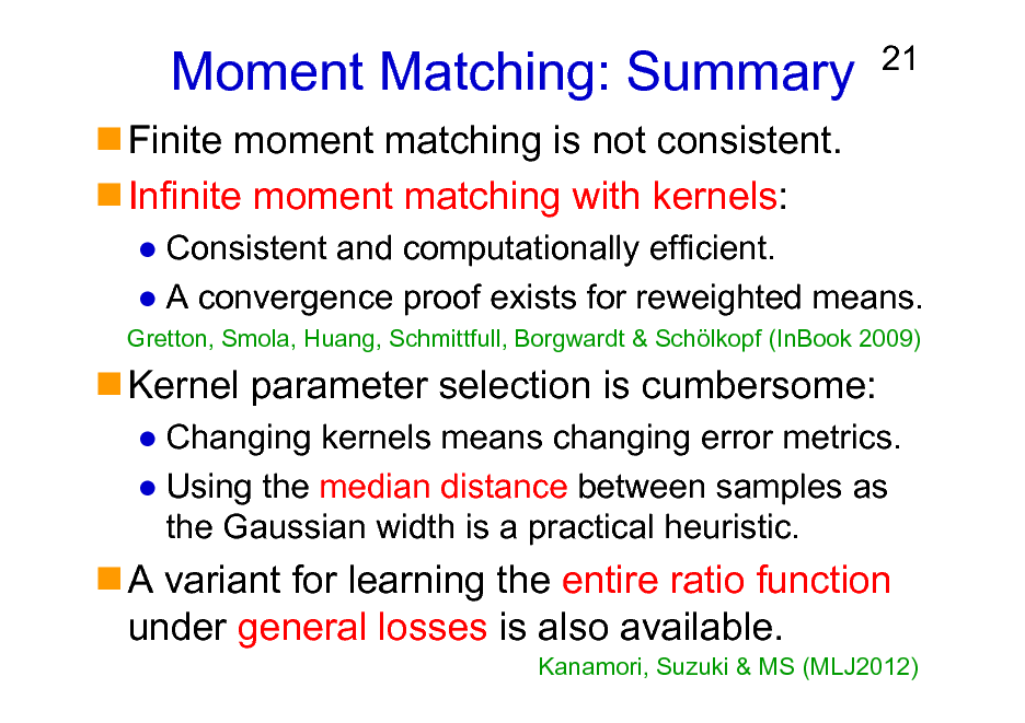
Moment Matching: Summary
Finite moment matching is not consistent. Infinite moment matching with kernels:
21
Consistent and computationally efficient. A convergence proof exists for reweighted means.
Gretton, Smola, Huang, Schmittfull, Borgwardt & Schlkopf (InBook 2009)
Kernel parameter selection is cumbersome:
Changing kernels means changing error metrics. Using the median distance between samples as the Gaussian width is a practical heuristic.
A variant for learning the entire ratio function under general losses is also available.
Kanamori, Suzuki & MS (MLJ2012)
21
Organization of This Lecture
1. Introduction 2. Methods of Density Ratio Estimation
A) B) C) D)
22
Probabilistic Classification Moment Matching Density Fitting Density-Ratio Fitting
3. Usage of Density Ratios 4. More on Density Ratio Estimation 5. Conclusions
22
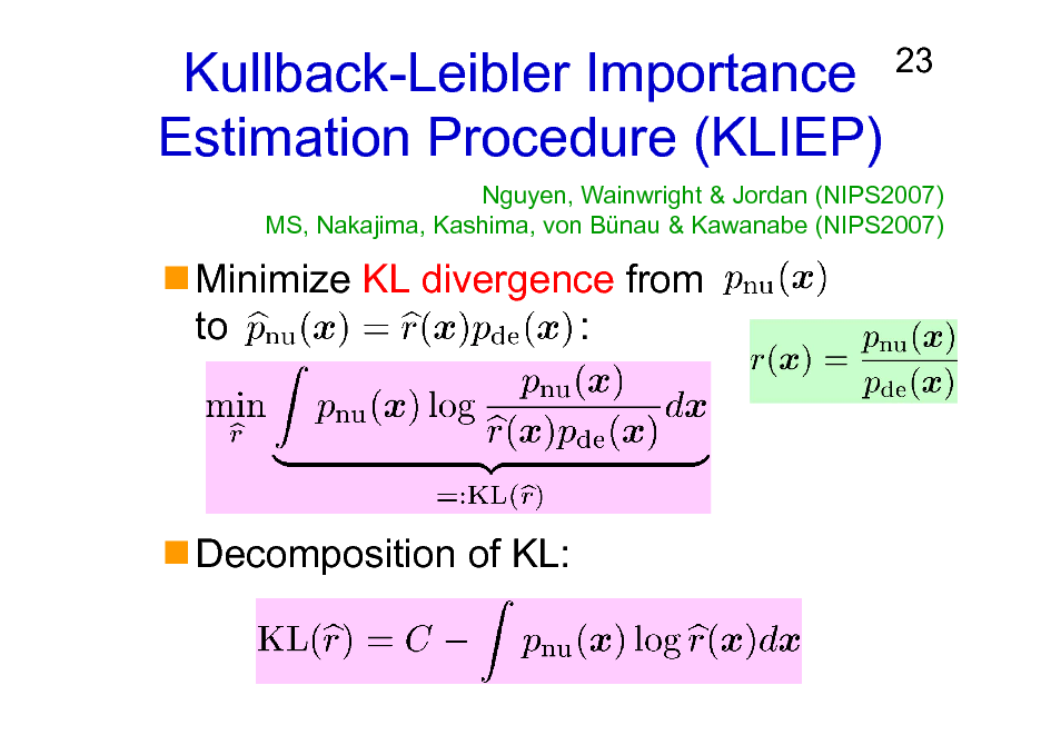
Kullback-Leibler Importance Estimation Procedure (KLIEP)
Minimize KL divergence from to :
23
Nguyen, Wainwright & Jordan (NIPS2007) MS, Nakajima, Kashima, von Bnau & Kawanabe (NIPS2007)
Decomposition of KL:
23
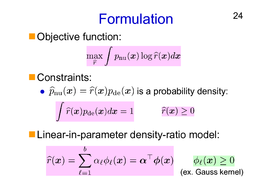
Formulation
Objective function:
24
Constraints:
is a probability density:
Linear-in-parameter density-ratio model:
(ex. Gauss kernel)
24
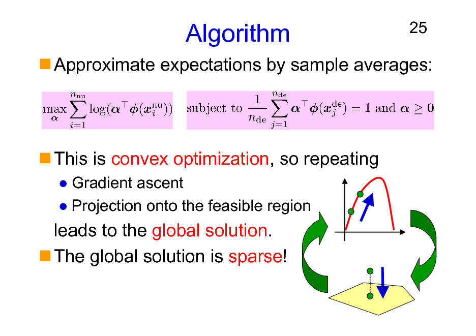
Algorithm
25
Approximate expectations by sample averages:
This is convex optimization, so repeating
Gradient ascent Projection onto the feasible region
leads to the global solution. The global solution is sparse!
25
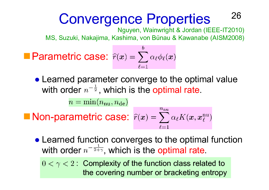
Nguyen, Wainwright & Jordan (IEEE-IT2010) MS, Suzuki, Nakajima, Kashima, von Bnau & Kawanabe (AISM2008)
Convergence Properties
26
Parametric case:
Learned parameter converge to the optimal value with order , which is the optimal rate.
Non-parametric case:
Learned function converges to the optimal function with order , which is the optimal rate.
: Complexity of the function class related to the covering number or bracketing entropy
26
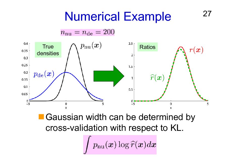
Numerical Example
True densities Ratios
27
Gaussian width can be determined by cross-validation with respect to KL.
27

Density Fitting under KL Divergence: Summary
Cross-validation is available for kernel parameter selection. Variations for various models exist:
28
Log-linear, Gaussian mixture, PCA mixture, etc.
Elaborate ratios such as can also be estimated. An unconstrained variant corresponds to maximizing a lower-bound of KL divergence.
Nguyen, Wainwright & Jordan (NIPS2007)
28
Organization of This Lecture
1. Introduction 2. Methods of Density Ratio Estimation
A) B) C) D)
29
Probabilistic Classification Moment Matching Density Fitting Density-Ratio Fitting
3. Usage of Density Ratios 4. More on Density Ratio Estimation 5. Conclusions
29
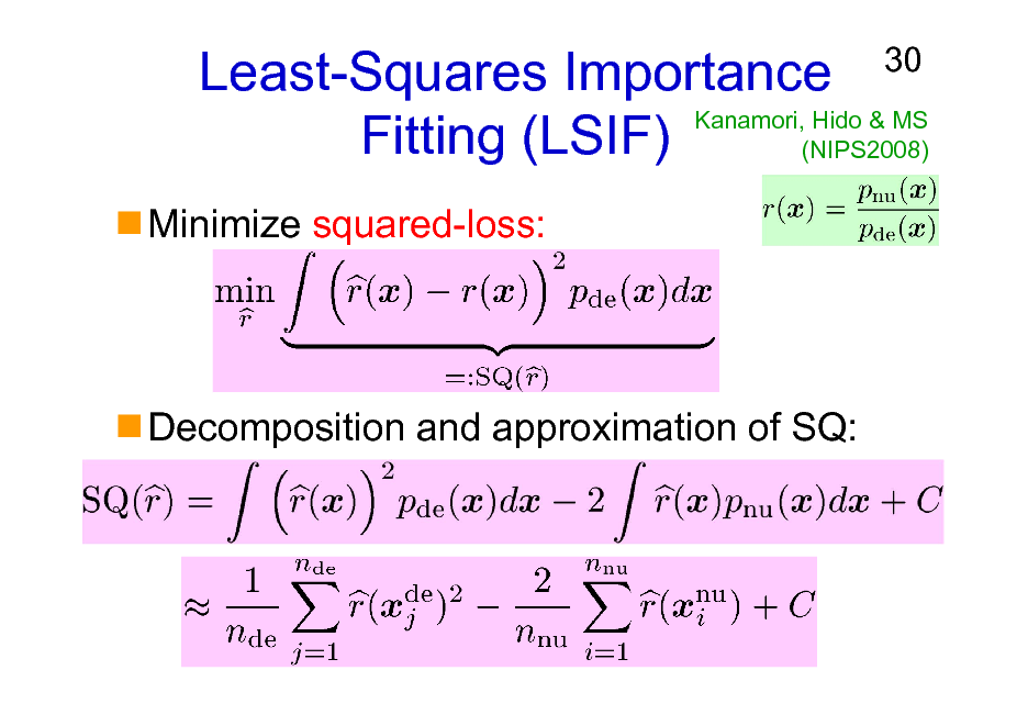
Least-Squares Importance Kanamori, Hido & MS Fitting (LSIF) (NIPS2008)
Minimize squared-loss:
30
Decomposition and approximation of SQ:
30
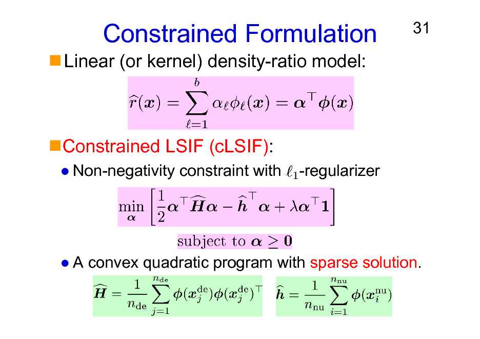
Constrained Formulation
Linear (or kernel) density-ratio model:
31
Constrained LSIF (cLSIF):
Non-negativity constraint with -regularizer
A convex quadratic program with sparse solution.
31
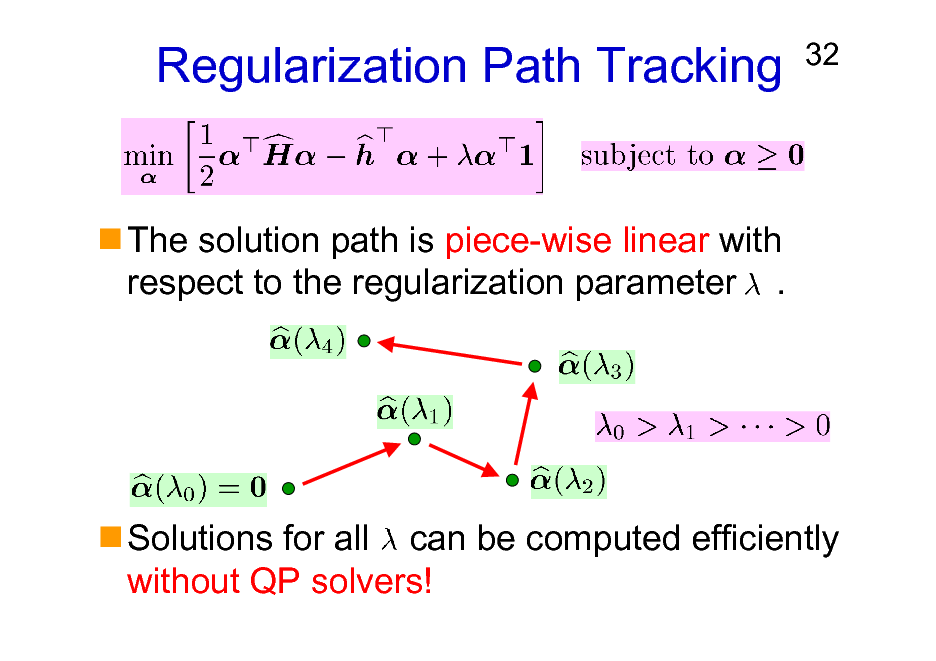
Regularization Path Tracking
32
The solution path is piece-wise linear with respect to the regularization parameter .
Solutions for all can be computed efficiently without QP solvers!
32
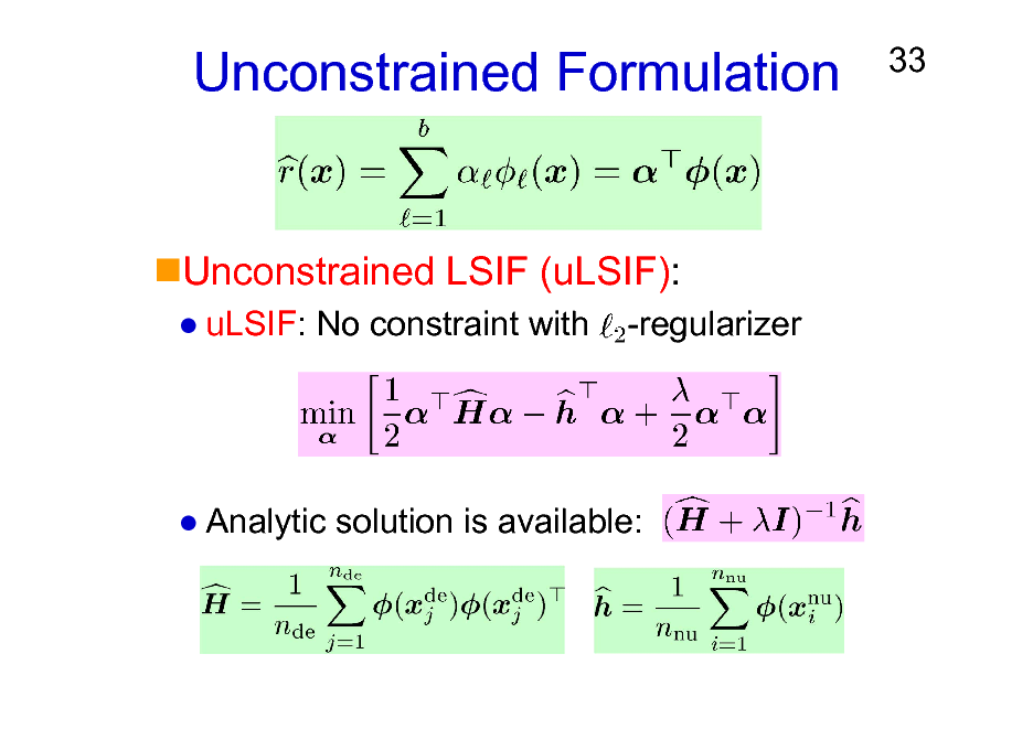
Unconstrained Formulation
33
Unconstrained LSIF (uLSIF):
uLSIF: No constraint with -regularizer
Analytic solution is available:
33
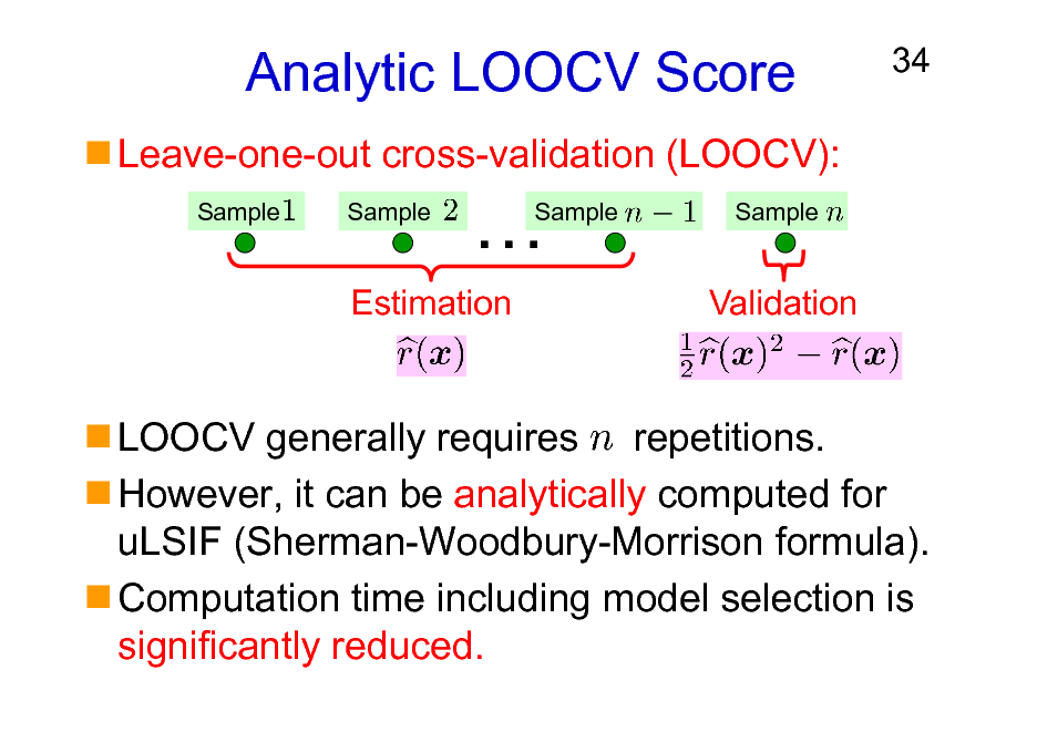
Analytic LOOCV Score
Leave-one-out cross-validation (LOOCV):
Sample Sample
34
Sample
Sample
Estimation
Validation
LOOCV generally requires repetitions. However, it can be analytically computed for uLSIF (Sherman-Woodbury-Morrison formula). Computation time including model selection is significantly reduced.
34
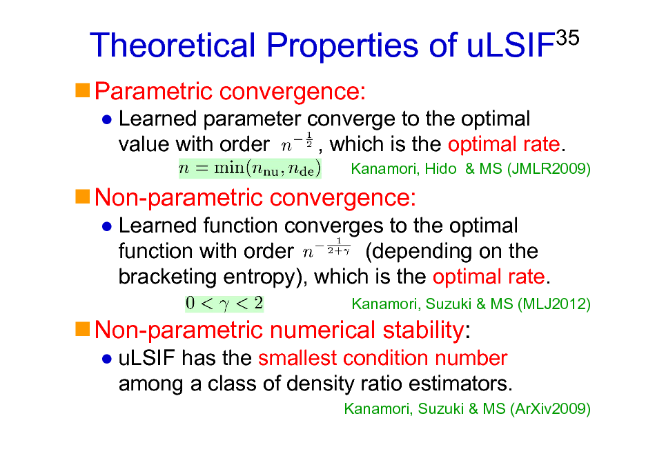
Theoretical Properties of uLSIF
Parametric convergence:
35
Learned parameter converge to the optimal value with order , which is the optimal rate.
Kanamori, Hido & MS (JMLR2009)
Non-parametric convergence:
Learned function converges to the optimal function with order (depending on the bracketing entropy), which is the optimal rate.
Kanamori, Suzuki & MS (MLJ2012)
Non-parametric numerical stability:
uLSIF has the smallest condition number among a class of density ratio estimators.
Kanamori, Suzuki & MS (ArXiv2009)
35
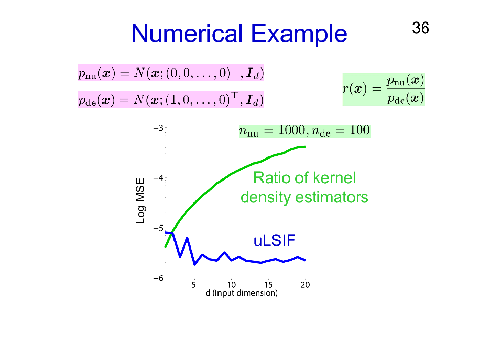
Numerical Example
36
Log MSE
Ratio of kernel density estimators uLSIF
36
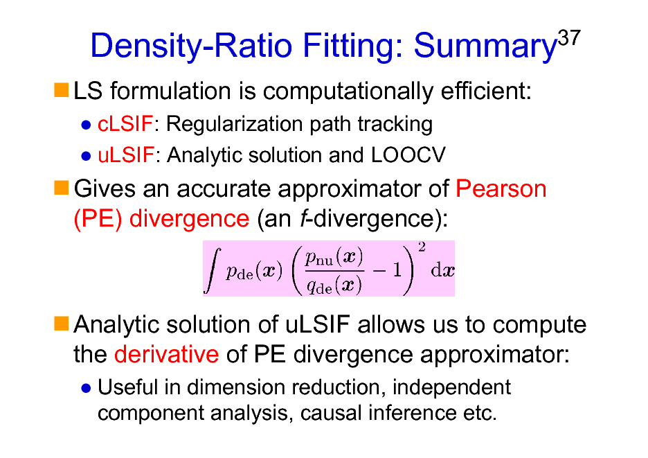
Density-Ratio Fitting: Summary
LS formulation is computationally efficient:
cLSIF: Regularization path tracking uLSIF: Analytic solution and LOOCV
37
Gives an accurate approximator of Pearson (PE) divergence (an f-divergence):
Analytic solution of uLSIF allows us to compute the derivative of PE divergence approximator:
Useful in dimension reduction, independent component analysis, causal inference etc.
37
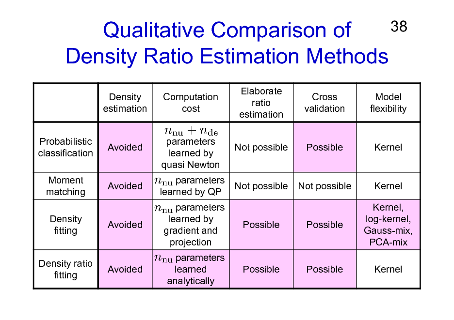
38 Qualitative Comparison of Density Ratio Estimation Methods
Density estimation Probabilistic classification Moment matching Density fitting Density ratio fitting Computation cost parameters learned by quasi Newton parameters learned by QP parameters learned by gradient and projection parameters learned analytically Elaborate ratio estimation Not possible Cross validation Model flexibility
Avoided
Possible
Kernel
Avoided
Not possible
Not possible
Kernel Kernel, log-kernel, Gauss-mix, PCA-mix Kernel
Avoided
Possible
Possible
Avoided
Possible
Possible
38
Organization of This Lecture
1. Introduction 2. Methods of Density Ratio Estimation 3. Usage of Density Ratios
A) B) C) D)
39
Importance sampling Distribution comparison Mutual information estimation Conditional probability estimation
4. More on Density Ratio Estimation 5. Conclusions
39
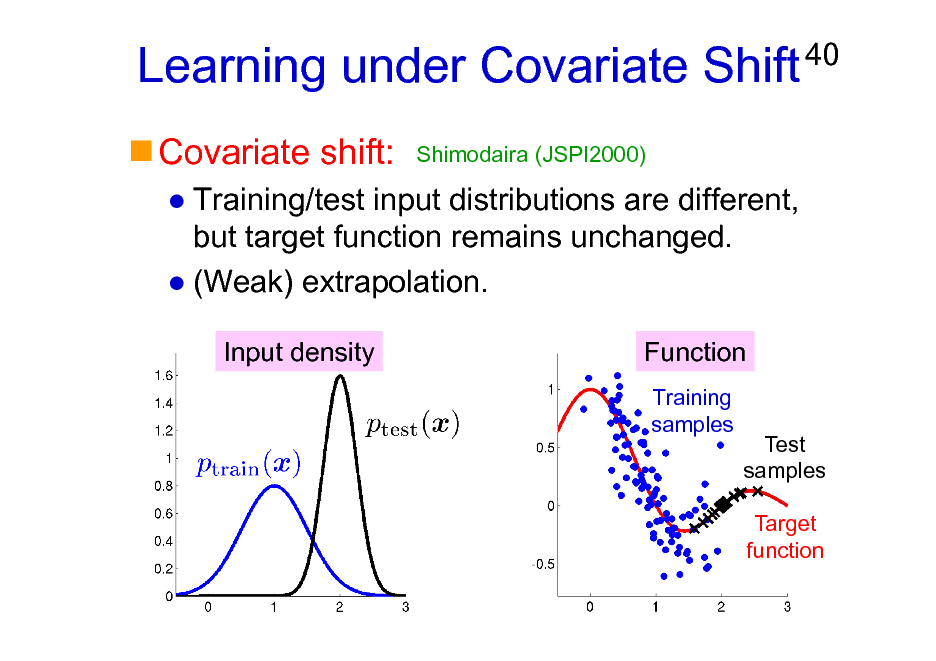
Learning under Covariate Shift
Covariate shift:
Shimodaira (JSPI2000)
40
Training/test input distributions are different, but target function remains unchanged. (Weak) extrapolation.
Input density Function
Training samples Test samples Target function
40
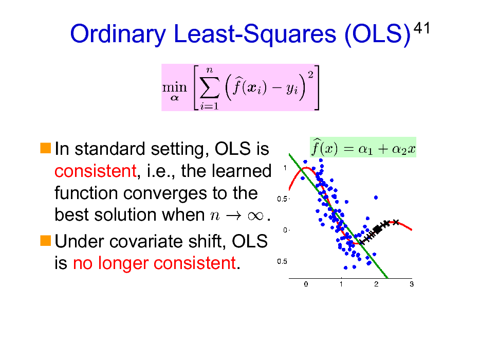
Ordinary Least-Squares (OLS)
41
In standard setting, OLS is consistent, i.e., the learned function converges to the best solution when . Under covariate shift, OLS is no longer consistent.
41
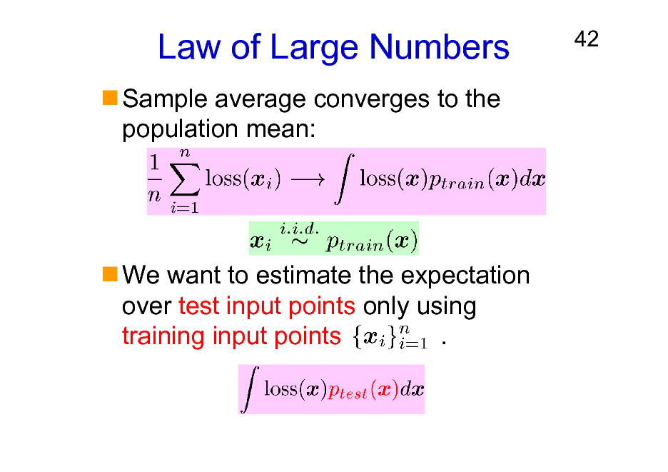
Law of Large Numbers
Sample average converges to the population mean:
42
We want to estimate the expectation over test input points only using training input points .
42
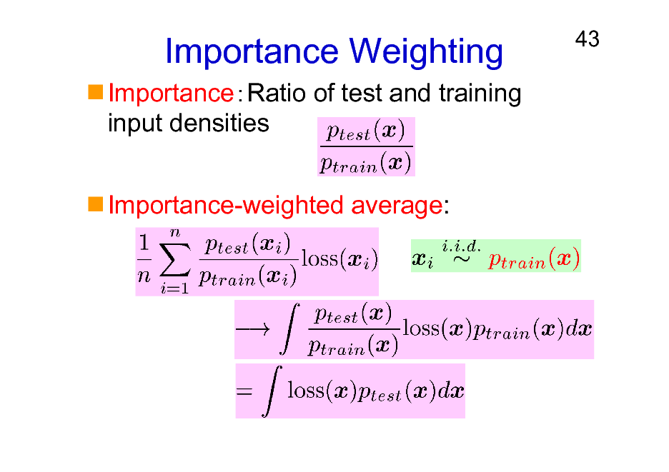
Importance Weighting
ImportanceRatio of test and training input densities Importance-weighted average:
43
43
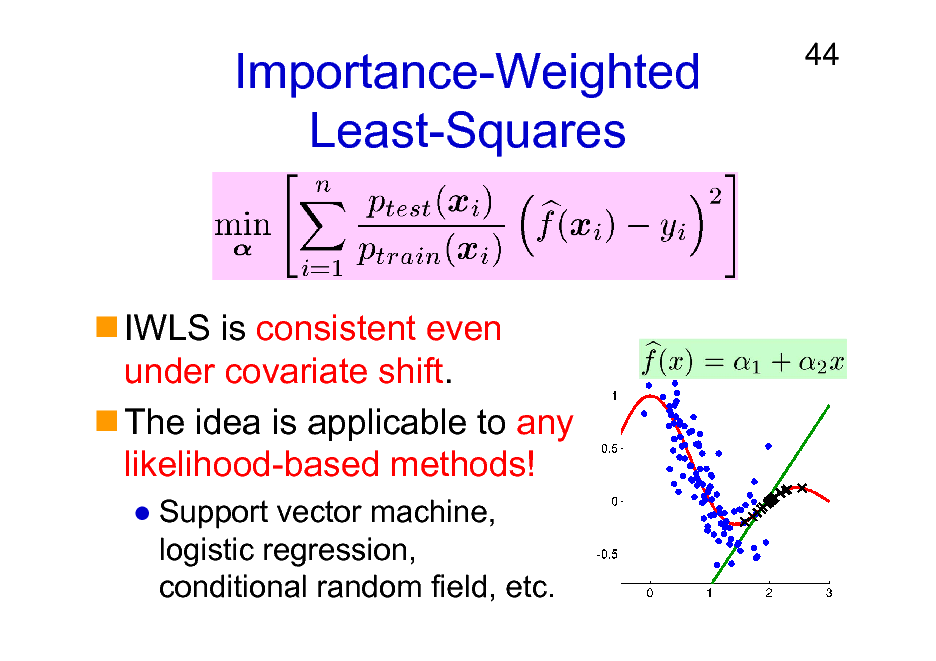
Importance-Weighted Least-Squares
44
IWLS is consistent even under covariate shift. The idea is applicable to any likelihood-based methods!
Support vector machine, logistic regression, conditional random field, etc.
44
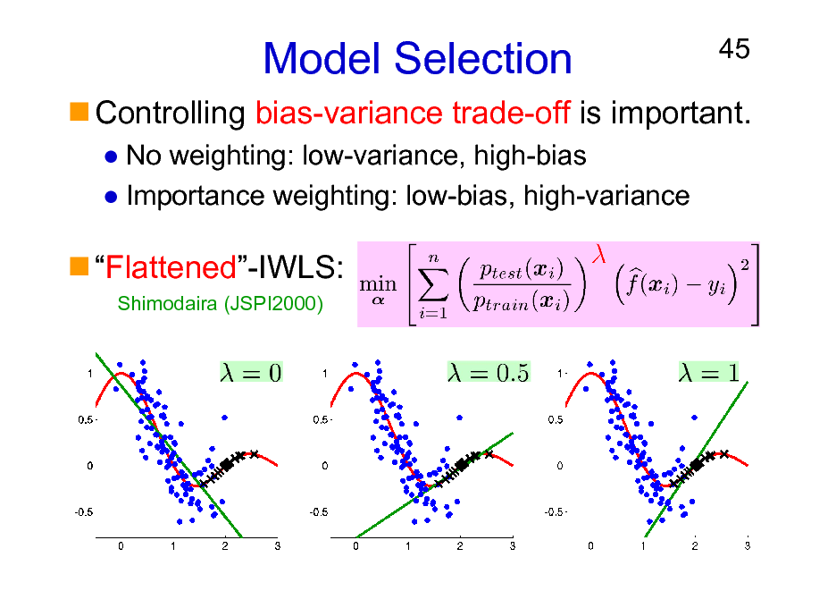
Model Selection
No weighting: low-variance, high-bias Importance weighting: low-bias, high-variance
45
Controlling bias-variance trade-off is important.
Flattened-IWLS:
Shimodaira (JSPI2000)
45
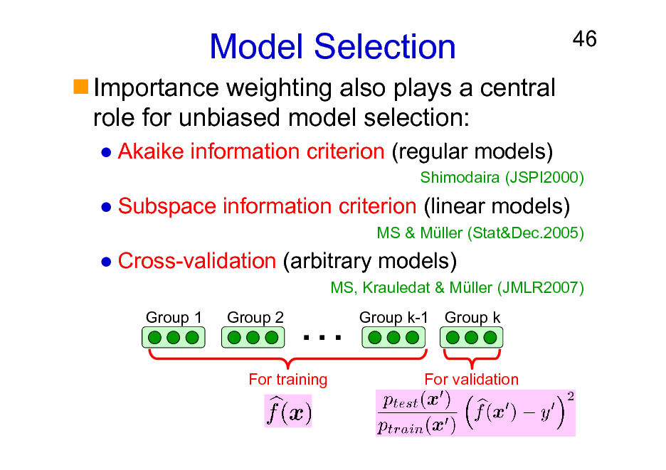
Model Selection
Importance weighting also plays a central role for unbiased model selection:
Akaike information criterion (regular models)
46
Shimodaira (JSPI2000)
Subspace information criterion (linear models)
MS & Mller (Stat&Dec.2005)
Cross-validation (arbitrary models)
MS, Krauledat & Mller (JMLR2007) Group 1 Group 2
Group k-1 Group k
For training
For validation
46
![Slide: Experiments: Speaker Identification
Yamada, MS & Matsui (SigPro2010)
47
NTT Japanese speech dataset: Matsui & Furui (ICASSP1993) Text-independent speaker identification accuracy for 10 male speakers. Kernel logistic regression (KLR) with sequence kernel.
Training data 9 months before Speech length 1.5 [sec] 3.0 [sec] 4.5 [sec] 1.5 [sec] 3.0 [sec] 4.5 [sec] 1.5 [sec] 3.0 [sec] 4.5 [sec] IWKLR+IWCV+KLIEP 91.0 % 95.0 % 97.7 % 91.0 % 95.3 % 97.4 % 94.8 % 97.9 % 98.8 % KLR+CV 88.2 % 92.9 % 96.1 % 87.7 % 91.1 % 93.4 % 91.7 % 96.3 % 98.3 %
6 months before
3 months before](https://yosinski.com/mlss12/media/slides/MLSS-2012-Sugiyama-Density-Ratio-Estimation-in-Machine-Learning_047.png)
Experiments: Speaker Identification
Yamada, MS & Matsui (SigPro2010)
47
NTT Japanese speech dataset: Matsui & Furui (ICASSP1993) Text-independent speaker identification accuracy for 10 male speakers. Kernel logistic regression (KLR) with sequence kernel.
Training data 9 months before Speech length 1.5 [sec] 3.0 [sec] 4.5 [sec] 1.5 [sec] 3.0 [sec] 4.5 [sec] 1.5 [sec] 3.0 [sec] 4.5 [sec] IWKLR+IWCV+KLIEP 91.0 % 95.0 % 97.7 % 91.0 % 95.3 % 97.4 % 94.8 % 97.9 % 98.8 % KLR+CV 88.2 % 92.9 % 96.1 % 87.7 % 91.1 % 93.4 % 91.7 % 96.3 % 98.3 %
6 months before
3 months before
47
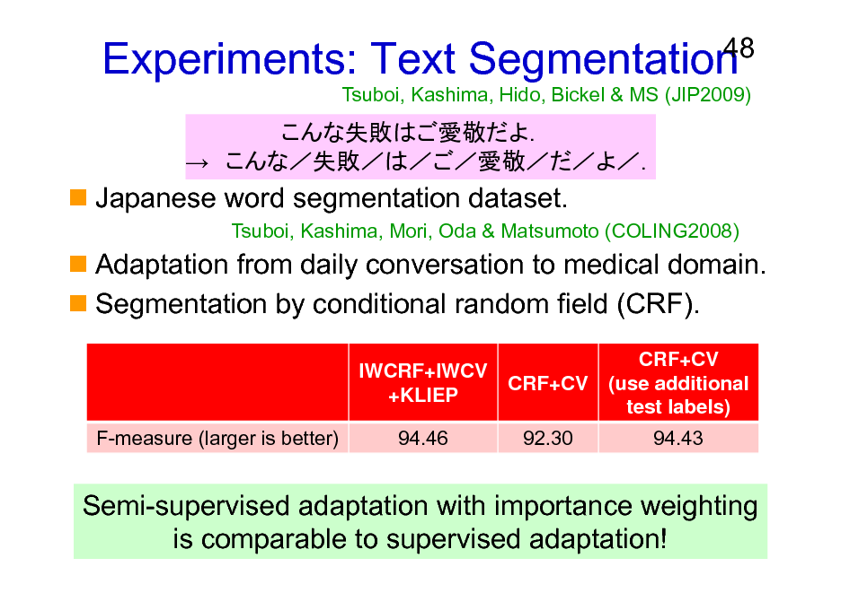
Experiments: Text Segmentation
48
Tsuboi, Kashima, Hido, Bickel & MS (JIP2009)
Japanese word segmentation dataset.
Tsuboi, Kashima, Mori, Oda & Matsumoto (COLING2008)
Adaptation from daily conversation to medical domain. Segmentation by conditional random field (CRF).
IWCRF+IWCV +KLIEP F-measure (larger is better) 94.46 CRF+CV 92.30 CRF+CV (use additional test labels) 94.43
Semi-supervised adaptation with importance weighting is comparable to supervised adaptation!
48
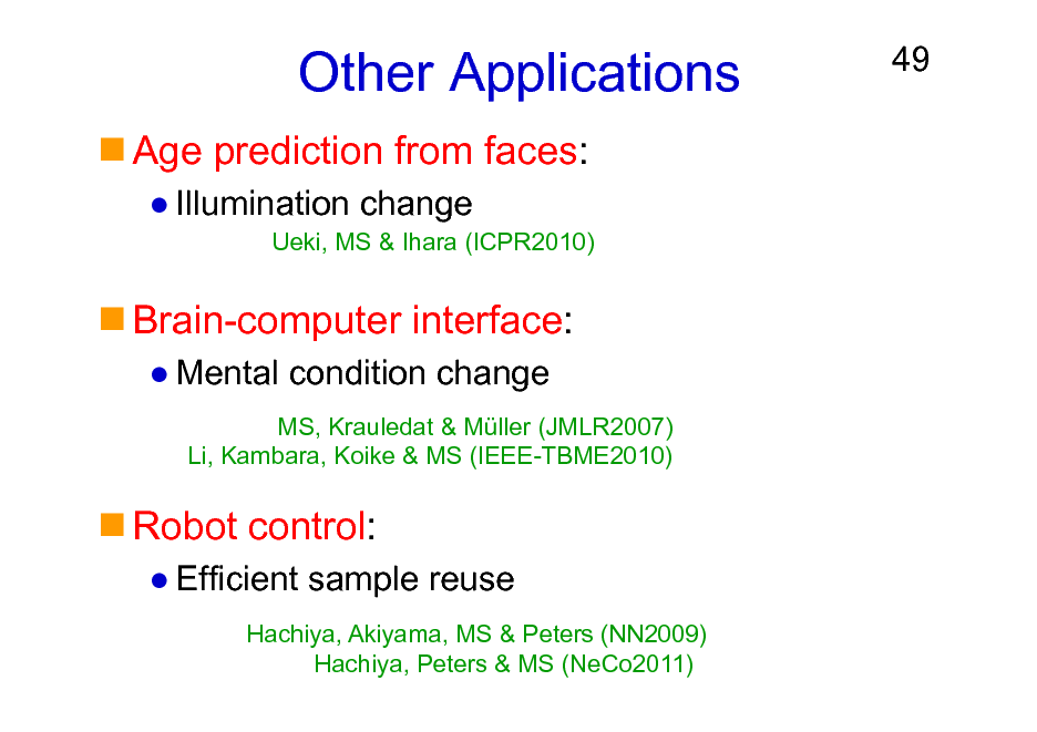
Other Applications
Age prediction from faces:
Illumination change
Ueki, MS & Ihara (ICPR2010)
49
Brain-computer interface:
Mental condition change
MS, Krauledat & Mller (JMLR2007) Li, Kambara, Koike & MS (IEEE-TBME2010)
Robot control:
Efficient sample reuse
Hachiya, Akiyama, MS & Peters (NN2009) Hachiya, Peters & MS (NeCo2011)
49
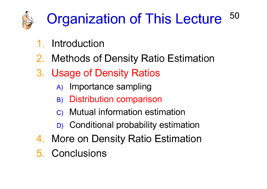
Organization of This Lecture
1. Introduction 2. Methods of Density Ratio Estimation 3. Usage of Density Ratios
A) B) C) D)
50
Importance sampling Distribution comparison Mutual information estimation Conditional probability estimation
4. More on Density Ratio Estimation 5. Conclusions
50
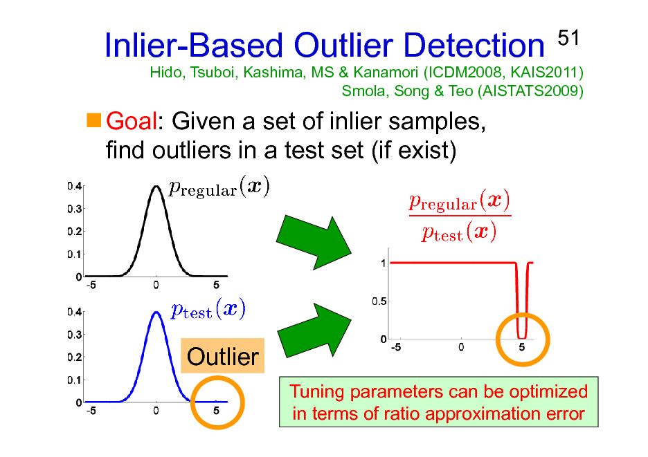
Inlier-Based Outlier Detection
Goal: Given a set of inlier samples, find outliers in a test set (if exist)
51
Hido, Tsuboi, Kashima, MS & Kanamori (ICDM2008, KAIS2011) Smola, Song & Teo (AISTATS2009)
Outlier
Tuning parameters can be optimized in terms of ratio approximation error
51
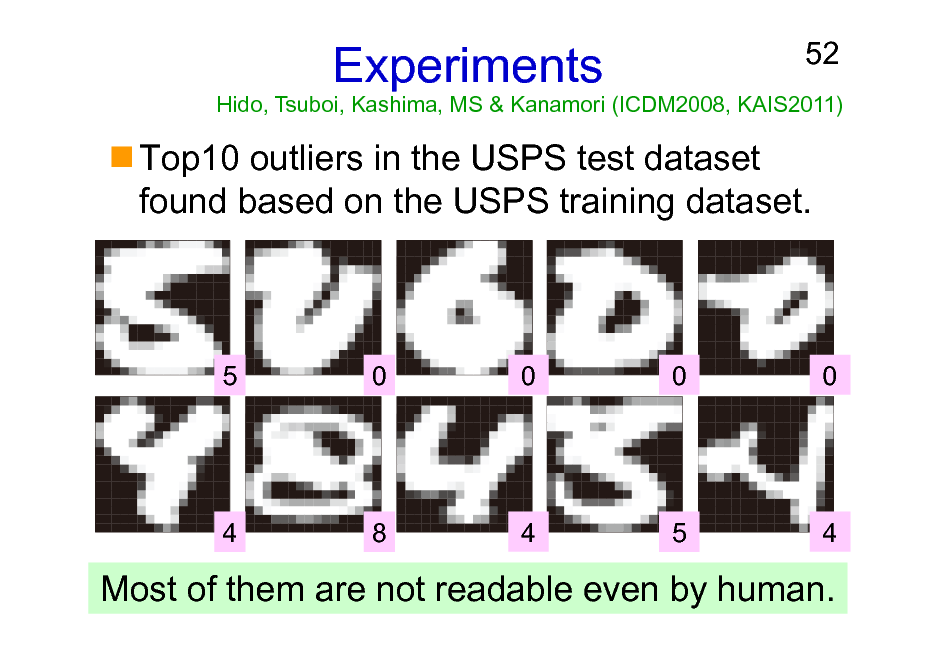
Experiments
52
Hido, Tsuboi, Kashima, MS & Kanamori (ICDM2008, KAIS2011)
Top10 outliers in the USPS test dataset found based on the USPS training dataset.
5
0
0
0
0
4
8
4
5
4
Most of them are not readable even by human.
52
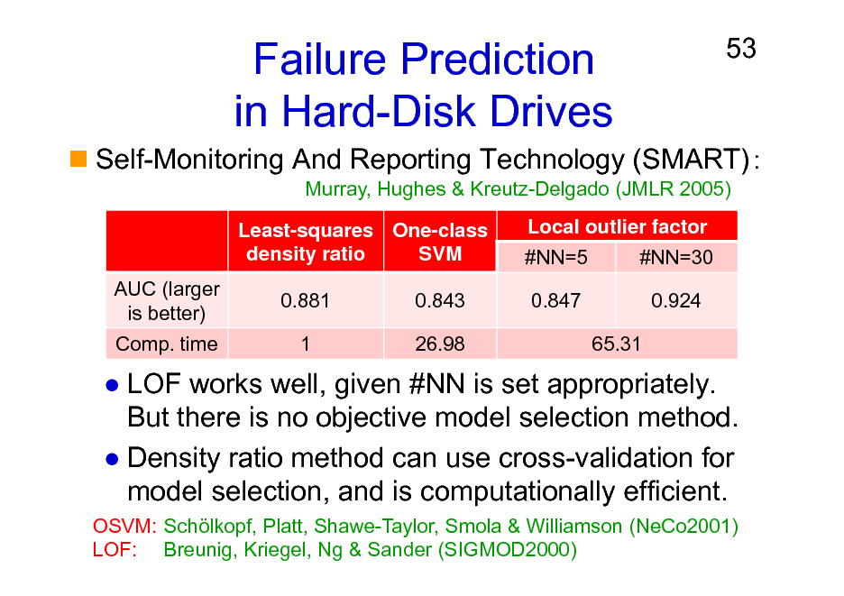
Failure Prediction in Hard-Disk Drives
Least-squares One-class density ratio SVM AUC (larger is better) Comp. time 0.881 1 0.843 26.98 Local outlier factor #NN=5 0.847 65.31 #NN=30 0.924
53
Self-Monitoring And Reporting Technology (SMART)
Murray, Hughes & Kreutz-Delgado (JMLR 2005)
LOF works well, given #NN is set appropriately. But there is no objective model selection method. Density ratio method can use cross-validation for model selection, and is computationally efficient.
OSVM: Schlkopf, Platt, Shawe-Taylor, Smola & Williamson (NeCo2001) LOF: Breunig, Kriegel, Ng & Sander (SIGMOD2000)
53
Other Applications
Steel plant diagnosis Printer roller quality control Loan customer inspection Sleep therapy
54
Hirata, Kawahara & MS (Patent2011) Takimoto, Matsugu & MS (DMSS2009) Hido, Tsuboi, Kashima, MS & Kanamori (KAIS2011) Kawahara & MS (SADM2012)
54
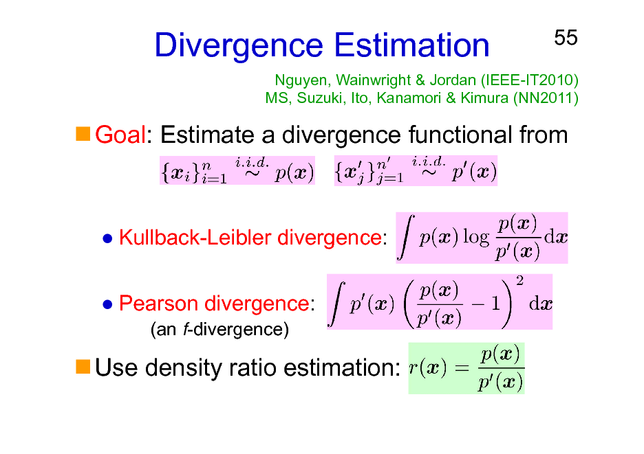
Divergence Estimation
55
Nguyen, Wainwright & Jordan (IEEE-IT2010) MS, Suzuki, Ito, Kanamori & Kimura (NN2011)
Goal: Estimate a divergence functional from
Kullback-Leibler divergence: Pearson divergence:
(an f-divergence)
Use density ratio estimation:
55
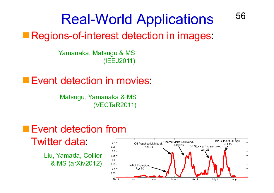
Real-World Applications
Regions-of-interest detection in images:
Yamanaka, Matsugu & MS (IEEJ2011)
56
Event detection in movies:
Matsugu, Yamanaka & MS (VECTaR2011)
Event detection from Twitter data:
Liu, Yamada, Collier & MS (arXiv2012)
56
Organization of This Lecture
1. Introduction 2. Methods of Density Ratio Estimation 3. Usage of Density Ratios
A) B) C) D)
57
Importance sampling Distribution comparison Mutual information estimation Conditional probability estimation
4. More on Density Ratio Estimation 5. Conclusions
57
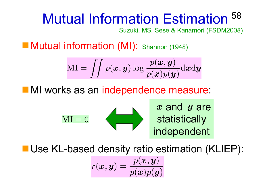
Mutual Information Estimation
Mutual information (MI):
Shannon (1948)
58
Suzuki, MS, Sese & Kanamori (FSDM2008)
MI works as an independence measure: and are statistically independent Use KL-based density ratio estimation (KLIEP):
58
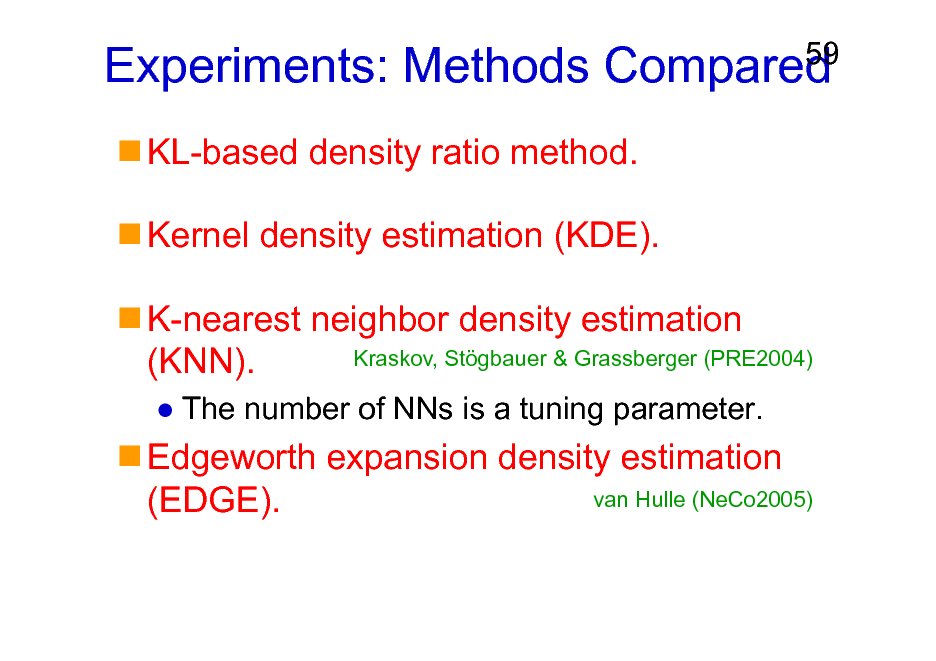
Experiments: Methods Compared
KL-based density ratio method. Kernel density estimation (KDE). K-nearest neighbor density estimation Kraskov, Stgbauer & Grassberger (PRE2004) (KNN).
The number of NNs is a tuning parameter.
59
Edgeworth expansion density estimation van Hulle (NeCo2005) (EDGE).
59
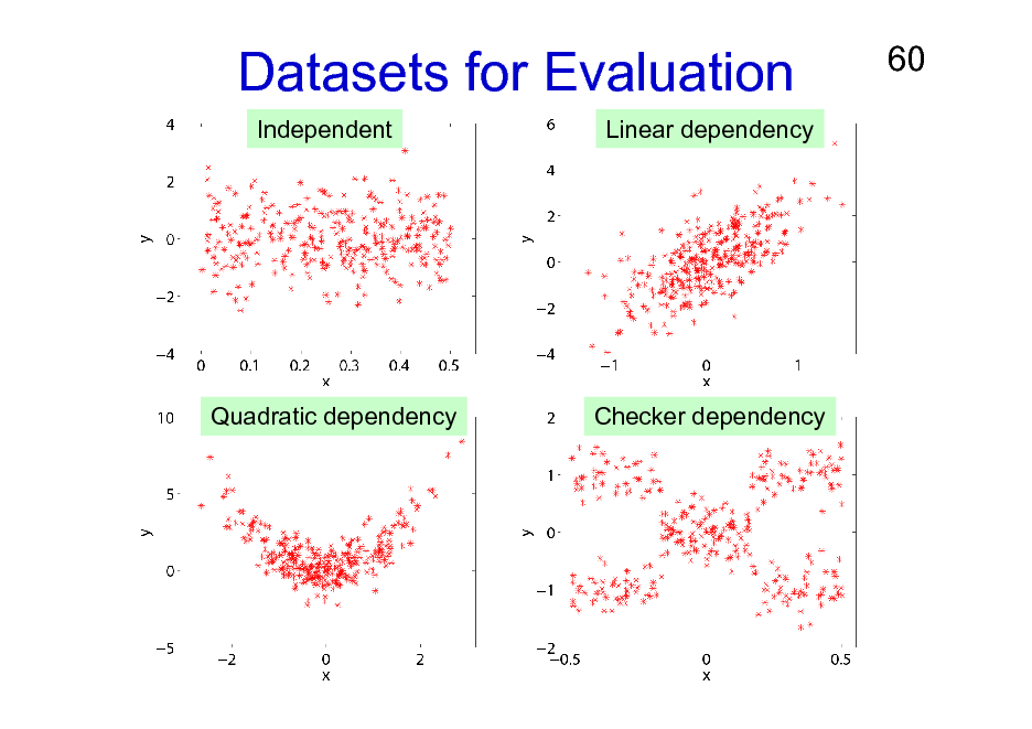
Datasets for Evaluation
Independent Linear dependency
60
Quadratic dependency
Checker dependency
60
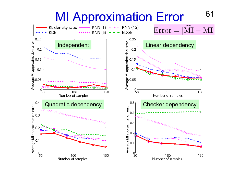
MI Approximation Error
Independent Linear dependency
61
Quadratic dependency
Checker dependency
61
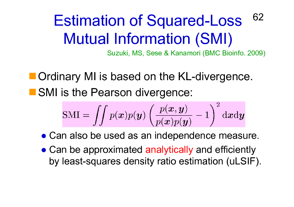
Estimation of Squared-Loss Mutual Information (SMI)
62
Suzuki, MS, Sese & Kanamori (BMC Bioinfo. 2009)
Ordinary MI is based on the KL-divergence. SMI is the Pearson divergence:
Can also be used as an independence measure. Can be approximated analytically and efficiently by least-squares density ratio estimation (uLSIF).
62
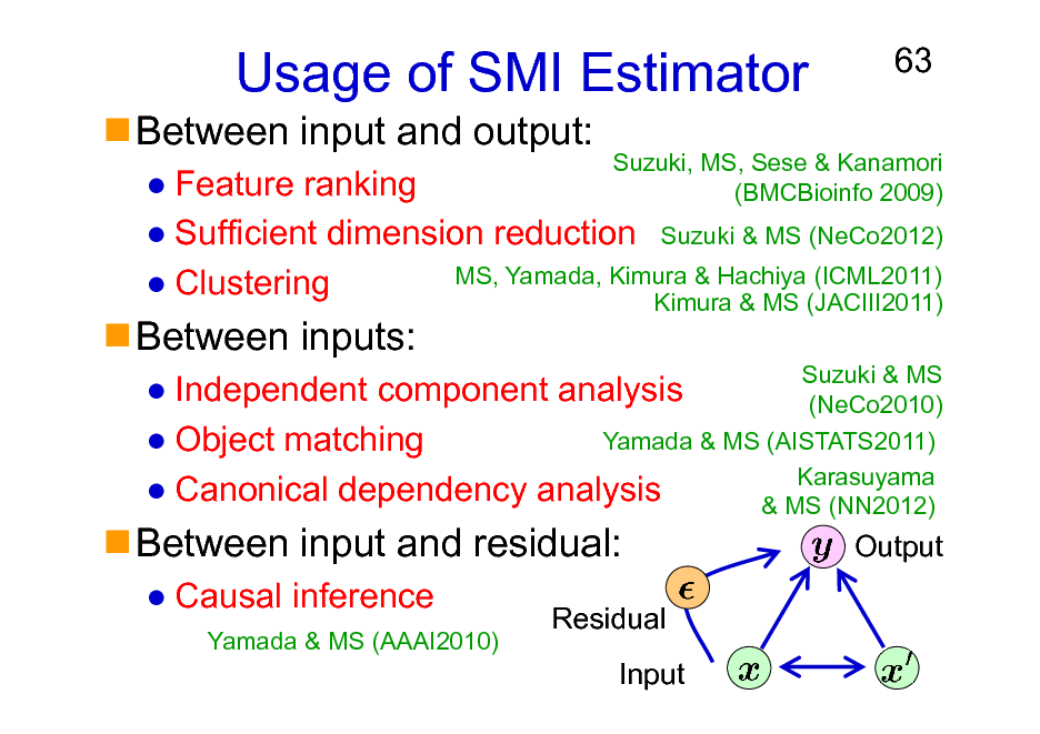
Usage of SMI Estimator
Between input and output:
63
Between inputs:
Feature ranking Sufficient dimension reduction Suzuki & MS (NeCo2012) MS, Yamada, Kimura & Hachiya (ICML2011) Clustering Kimura & MS (JACIII2011)
Suzuki & MS Independent component analysis (NeCo2010) Yamada & MS (AISTATS2011) Object matching Karasuyama Canonical dependency analysis & MS (NN2012)
Suzuki, MS, Sese & Kanamori (BMCBioinfo 2009)
Between input and residual:
Causal inference
Yamada & MS (AAAI2010)
Output
Residual Input
63
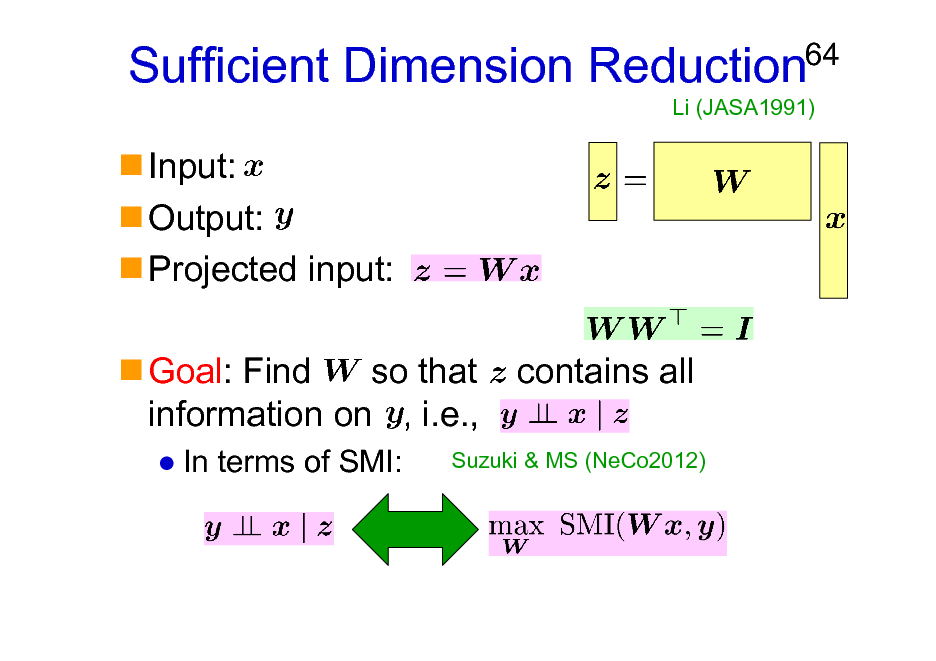
Sufficient Dimension Reduction
Input: Output: Projected input: Goal: Find so that information on , i.e.,
In terms of SMI:
64
Li (JASA1991)
contains all
Suzuki & MS (NeCo2012)
64
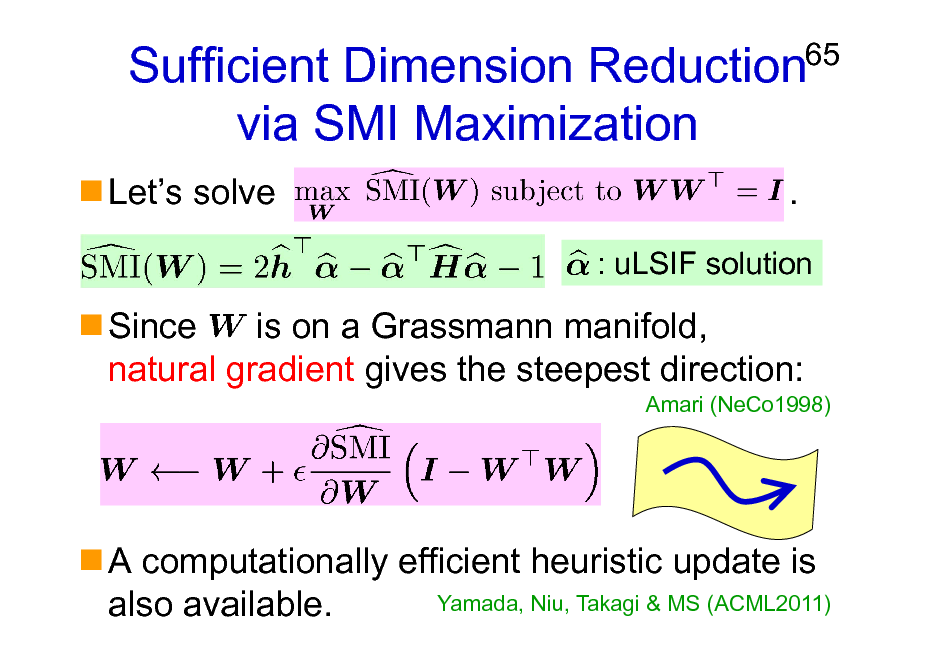
Sufficient Dimension Reduction via SMI Maximization
Lets solve .
65
: uLSIF solution
Since is on a Grassmann manifold, natural gradient gives the steepest direction:
Amari (NeCo1998)
A computationally efficient heuristic update is Yamada, Niu, Takagi & MS (ACML2011) also available.
65
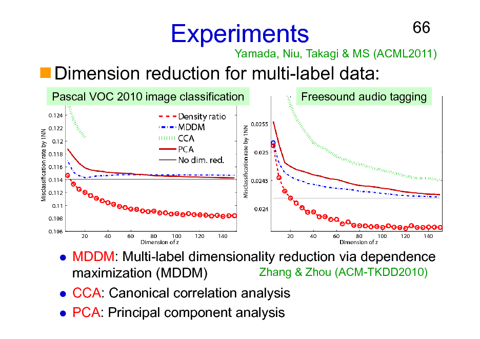
Experiments
Pascal VOC 2010 image classification
66
Yamada, Niu, Takagi & MS (ACML2011)
Dimension reduction for multi-label data:
Freesound audio tagging
MDDM: Multi-label dimensionality reduction via dependence Zhang & Zhou (ACM-TKDD2010) maximization (MDDM) CCA: Canonical correlation analysis PCA: Principal component analysis
66
Organization of This Lecture
1. Introduction 2. Methods of Density Ratio Estimation 3. Usage of Density Ratios
A) B) C) D)
67
Importance sampling Distribution comparison Mutual information estimation Conditional probability estimation
4. More on Density Ratio Estimation 5. Conclusions
67
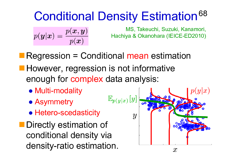
Conditional Density Estimation
Regression = Conditional mean estimation However, regression is not informative enough for complex data analysis:
Multi-modality Asymmetry Hetero-scedasticity
68
MS, Takeuchi, Suzuki, Kanamori, Hachiya & Okanohara (IEICE-ED2010)
Directly estimation of conditional density via density-ratio estimation.
68
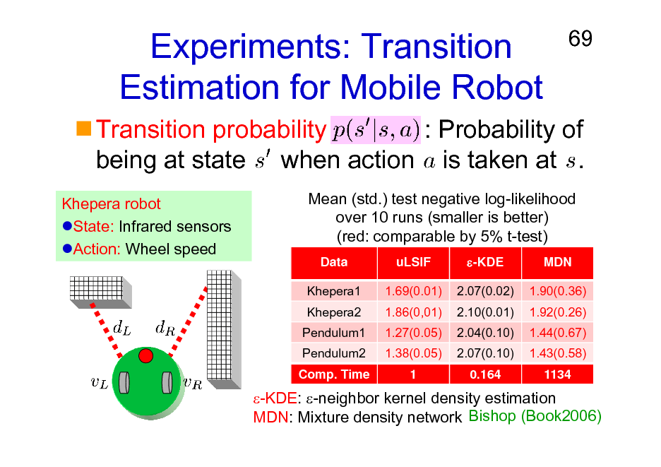
Experiments: Transition Estimation for Mobile Robot
69
Transition probability : Probability of being at state when action is taken at .
Khepera robot State: Infrared sensors Action: Wheel speed Mean (std.) test negative log-likelihood over 10 runs (smaller is better) (red: comparable by 5% t-test)
Data Khepera1 Khepera2 Pendulum1 Pendulum2 Comp. Time uLSIF 1.69(0.01) 1.86(0,01) 1.27(0.05) 1.38(0.05) 1 -KDE 2.07(0.02) 2.10(0.01) 2.04(0.10) 2.07(0.10) 0.164 MDN 1.90(0.36) 1.92(0.26) 1.44(0.67) 1.43(0.58) 1134
-KDE: -neighbor kernel density estimation MDN: Mixture density network Bishop (Book2006)
69
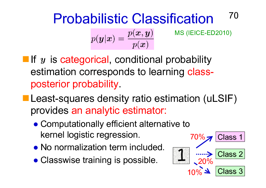
Probabilistic Classification
70
MS (IEICE-ED2010)
If is categorical, conditional probability estimation corresponds to learning classposterior probability. Least-squares density ratio estimation (uLSIF) provides an analytic estimator:
Computationally efficient alternative to kernel logistic regression. 70% Class 1 No normalization term included. Class 2 Classwise training is possible. 20%
10% Class 3
70
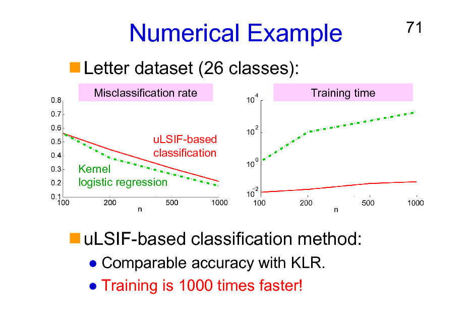
Numerical Example
Letter dataset (26 classes):
Misclassification rate Training time
71
uLSIF-based classification Kernel logistic regression
uLSIF-based classification method:
Comparable accuracy with KLR. Training is 1000 times faster!
71
![Slide: More Experiments
Dataset Aeroplane Bicycle Bird Boat Bottle Bus Car Cat Chair Cow Diningtable Dog Horse Motorbike Person Pottedplant Sheep Sofa Train Tvmonitor Training time [sec] uLSIF 82.6(1.0) 77.7(1.7) 68.7(2.0) 74.4(2.0) 65.4(1.8) 85.4(1.4) 73.0(0.8) 73.6(1.4) 71.0(1.0) 71.7(3.2) 75.0(1.6) 69.6(1.0) 64.4(2.5) 77.0(1.7) 67.6(0.9) 66.2(2.6) 77.8(1.6) 67.4(2.7) 79.2(1.3) 76.7(2.2) 0.7 KLR 83.0(1.3) 76.6(3.4) 70.8(2.2) 72.8(2.6) 62.1(4.3) 85.6(1.4) 72.1(1.2) 74.1(1.7) 70.5(1.0) 69.3(3.6) 71.4(2.7) 69.4(1.8) 61.2(3.2) 75.9(3.3) 67.0(0.8) 61.9(3.2) 74.0(3.8) 65.4(4.6 78.4(3.0) 76.6(2.3) 24.6
72
Yamada, MS, Wichern & Simm (IEICE2011)
Pascal VOC 2010 image classification: Mean AUC (std) over 50 runs (red: comparable by 5% t-test) Freesound audio tagging: Mean AUC (std) over 50 runs
uLSIF AUC Training time [sec] 70.1(9.6) 0.005
KLR 66.7(10.3) 0.612](https://yosinski.com/mlss12/media/slides/MLSS-2012-Sugiyama-Density-Ratio-Estimation-in-Machine-Learning_072.png)
More Experiments
Dataset Aeroplane Bicycle Bird Boat Bottle Bus Car Cat Chair Cow Diningtable Dog Horse Motorbike Person Pottedplant Sheep Sofa Train Tvmonitor Training time [sec] uLSIF 82.6(1.0) 77.7(1.7) 68.7(2.0) 74.4(2.0) 65.4(1.8) 85.4(1.4) 73.0(0.8) 73.6(1.4) 71.0(1.0) 71.7(3.2) 75.0(1.6) 69.6(1.0) 64.4(2.5) 77.0(1.7) 67.6(0.9) 66.2(2.6) 77.8(1.6) 67.4(2.7) 79.2(1.3) 76.7(2.2) 0.7 KLR 83.0(1.3) 76.6(3.4) 70.8(2.2) 72.8(2.6) 62.1(4.3) 85.6(1.4) 72.1(1.2) 74.1(1.7) 70.5(1.0) 69.3(3.6) 71.4(2.7) 69.4(1.8) 61.2(3.2) 75.9(3.3) 67.0(0.8) 61.9(3.2) 74.0(3.8) 65.4(4.6 78.4(3.0) 76.6(2.3) 24.6
72
Yamada, MS, Wichern & Simm (IEICE2011)
Pascal VOC 2010 image classification: Mean AUC (std) over 50 runs (red: comparable by 5% t-test) Freesound audio tagging: Mean AUC (std) over 50 runs
uLSIF AUC Training time [sec] 70.1(9.6) 0.005
KLR 66.7(10.3) 0.612
72
Other Applications
Action recognition from accelerometer
Hachiya, MS & Ueda (Neurocomputing 2011)
73
Age prediction from faces
Ueki, MS, Ihara & Fujita (ACPR2011)
73

Organization of This Lecture
1. 2. 3. 4. Introduction Methods of Density Ratio Estimation Usage of Density Ratios More on Density Ratio Estimation
A) B) C)
74
Unified Framework Dimensionality Reduction Relative Density Ratios
5. Conclusions
74
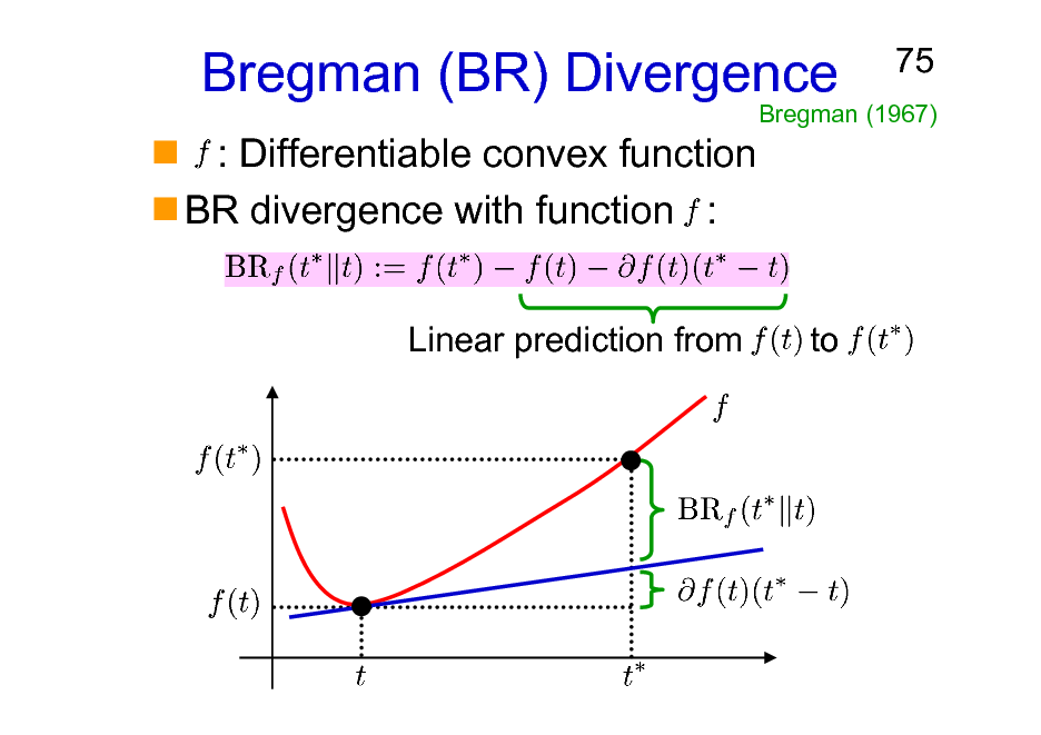
Bregman (BR) Divergence
: Differentiable convex function BR divergence with function :
Linear prediction from
75
Bregman (1967)
to
75
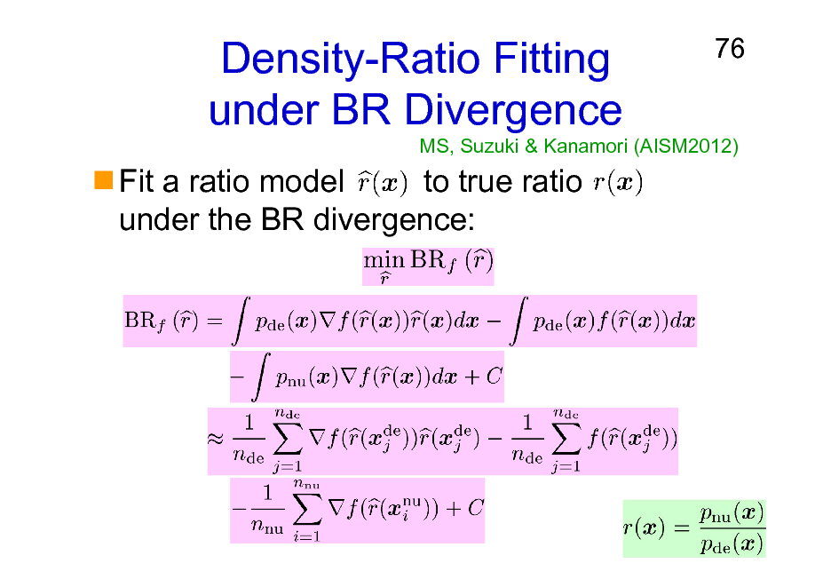
Density-Ratio Fitting under BR Divergence
Fit a ratio model to true ratio under the BR divergence:
76
MS, Suzuki & Kanamori (AISM2012)
76
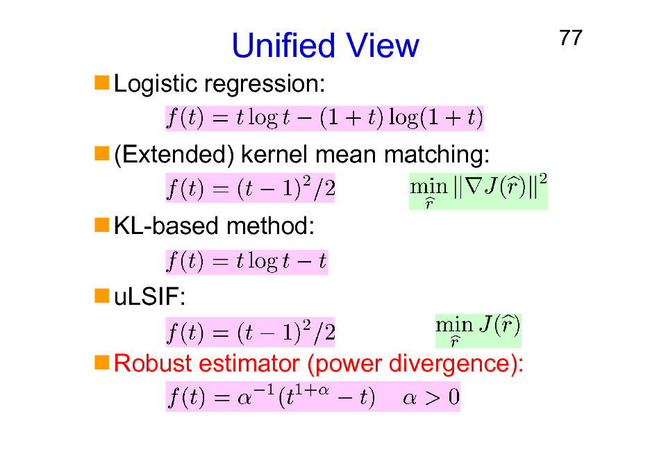
Unified View
Logistic regression: (Extended) kernel mean matching: KL-based method: uLSIF: Robust estimator (power divergence):
77
77
Organization of This Lecture
1. 2. 3. 4. Introduction Methods of Density Ratio Estimation Usage of Density Ratios More on Density Ratio Estimation
A) B) C)
78
Unified Framework Dimensionality Reduction Relative Density Ratios
5. Conclusions
78
Direct Density-Ratio Estimation with Dimensionality Reduction (D3)
Directly density-ratio estimation without density estimation is promising. However, for high-dimensional data, density-ratio estimation is still challenging. We combine direct density-ratio estimation with dimensionality reduction!
79
79
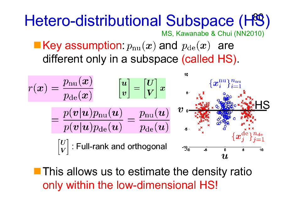
Hetero-distributional Subspace (HS)
MS, Kawanabe & Chui (NN2010)
80
Key assumption: and are different only in a subspace (called HS).
HS
: Full-rank and orthogonal
This allows us to estimate the density ratio only within the low-dimensional HS!
80
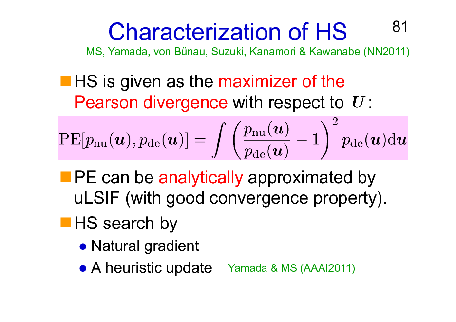
Characterization of HS
HS is given as the maximizer of the Pearson divergence with respect to :
81
MS, Yamada, von Bnau, Suzuki, Kanamori & Kawanabe (NN2011)
PE can be analytically approximated by uLSIF (with good convergence property). HS search by
Natural gradient A heuristic update
Yamada & MS (AAAI2011)
81
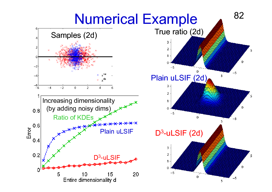
Numerical Example
Samples (2d) True ratio (2d)
82
Plain uLSIF (2d)
Increasing dimensionality (by adding noisy dims) Ratio of KDEs Plain uLSIF
D3-uLSIF (2d)
D3-uLSIF
82
Organization of This Lecture
1. 2. 3. 4. Introduction Methods of Density Ratio Estimation Usage of Density Ratios More on Density Ratio Estimation
A) B) C)
83
Unified Framework Dimensionality Reduction Relative Density Ratios
5. Conclusions
83
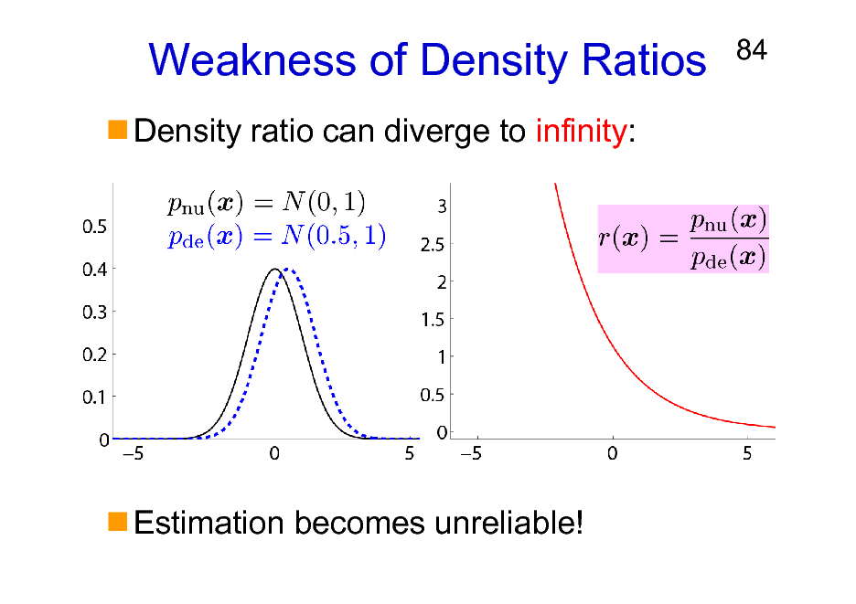
Weakness of Density Ratios
Density ratio can diverge to infinity:
84
Estimation becomes unreliable!
84
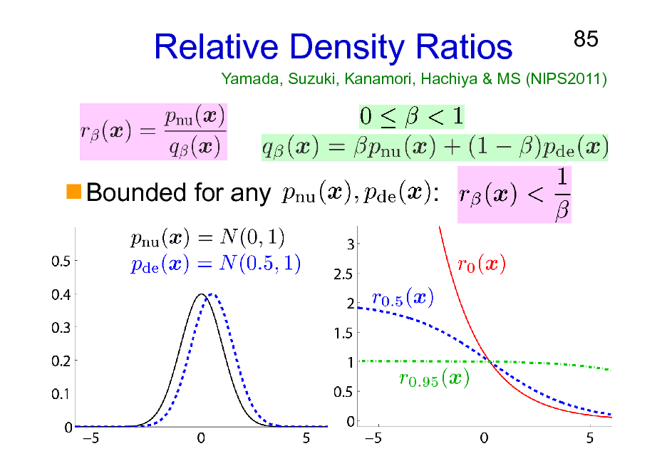
Relative Density Ratios
85
Yamada, Suzuki, Kanamori, Hachiya & MS (NIPS2011)
Bounded for any
:
85
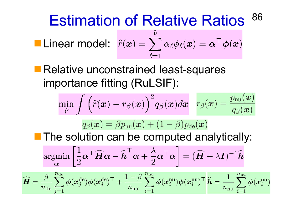
Estimation of Relative Ratios
Linear model: Relative unconstrained least-squares importance fitting (RuLSIF):
86
The solution can be computed analytically:
86
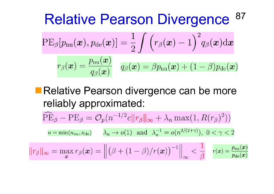
Relative Pearson Divergence
87
Relative Pearson divergence can be more reliably approximated:
87
Organization of This Lecture
1. 2. 3. 4. 5. Introduction Methods of Density Ratio Estimation Usage of Density Ratios More on Density Ratio Estimation Conclusions
88
88
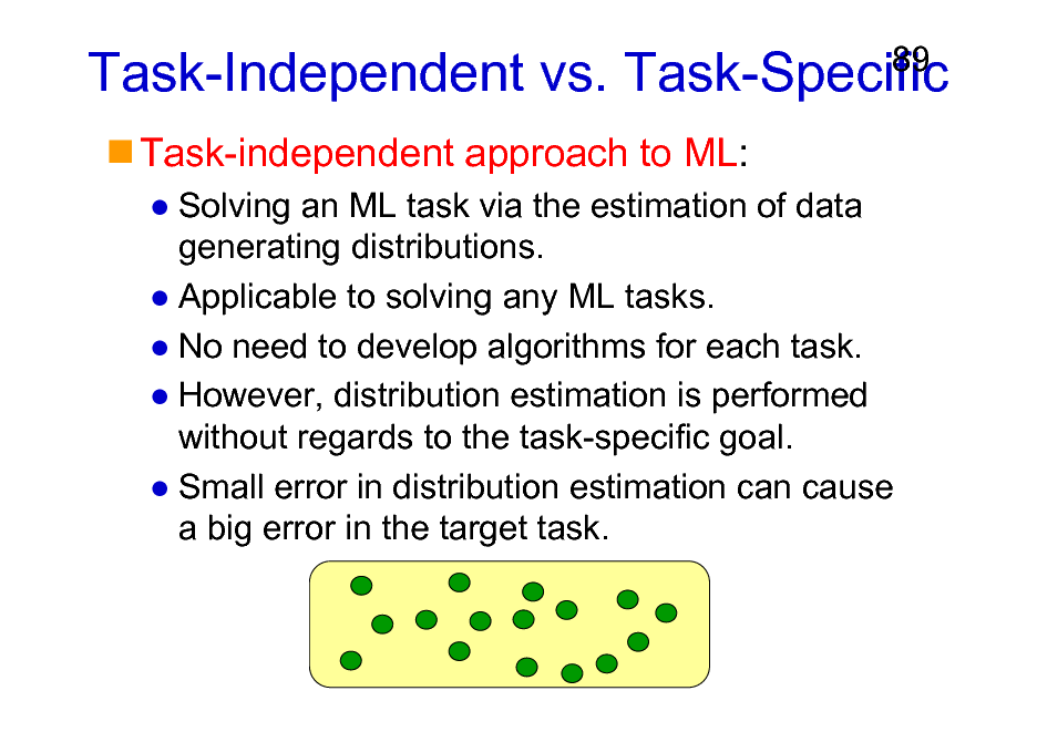
Task-Independent vs. Task-Specific
Task-independent approach to ML:
Solving an ML task via the estimation of data generating distributions. Applicable to solving any ML tasks. No need to develop algorithms for each task. However, distribution estimation is performed without regards to the task-specific goal. Small error in distribution estimation can cause a big error in the target task.
89
89
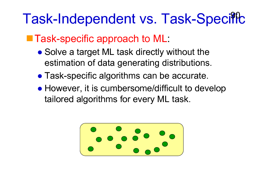
Task-Independent vs. Task-Specific
Task-specific approach to ML:
Solve a target ML task directly without the estimation of data generating distributions. Task-specific algorithms can be accurate. However, it is cumbersome/difficult to develop tailored algorithms for every ML task.
90
90
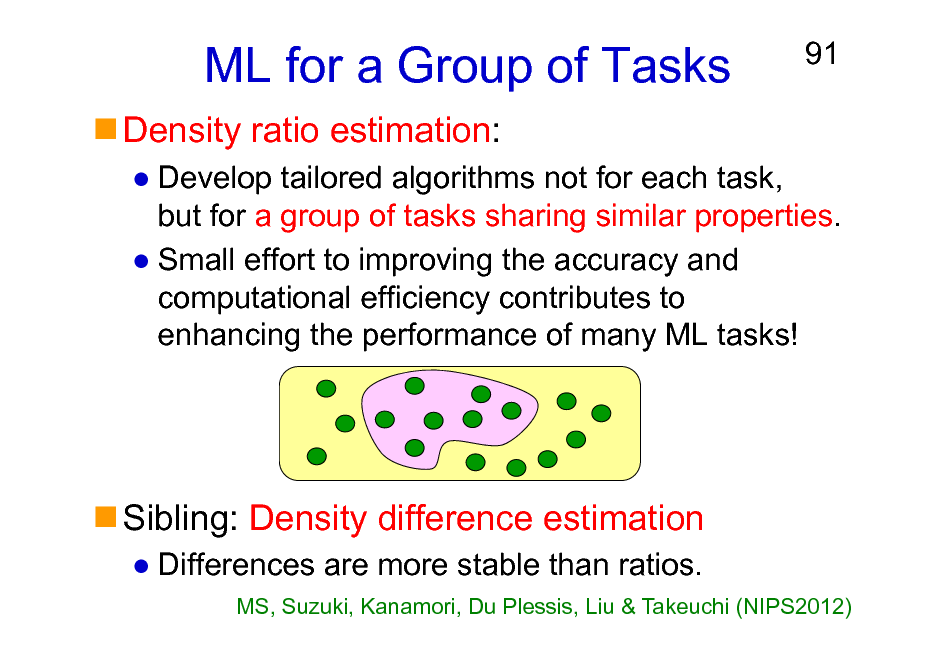
ML for a Group of Tasks
Density ratio estimation:
91
Develop tailored algorithms not for each task, but for a group of tasks sharing similar properties. Small effort to improving the accuracy and computational efficiency contributes to enhancing the performance of many ML tasks!
Sibling: Density difference estimation
Differences are more stable than ratios.
MS, Suzuki, Kanamori, Du Plessis, Liu & Takeuchi (NIPS2012)
91
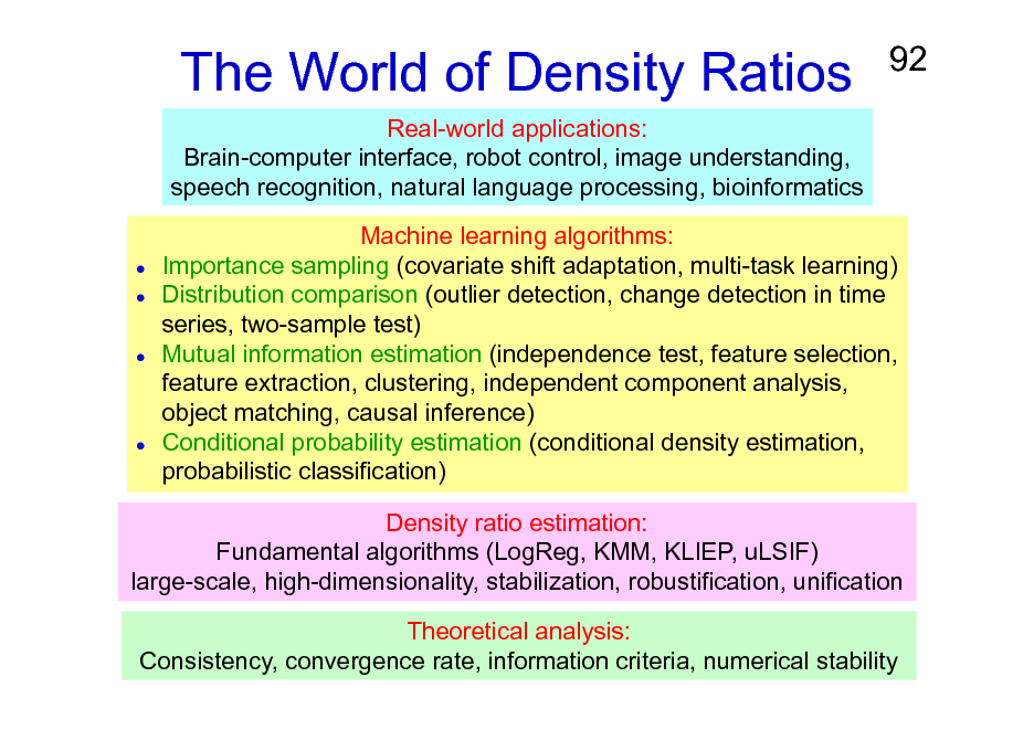
The World of Density Ratios
Real-world applications: Brain-computer interface, robot control, image understanding, speech recognition, natural language processing, bioinformatics
92
Machine learning algorithms: Importance sampling (covariate shift adaptation, multi-task learning) Distribution comparison (outlier detection, change detection in time series, two-sample test) Mutual information estimation (independence test, feature selection, feature extraction, clustering, independent component analysis, object matching, causal inference) Conditional probability estimation (conditional density estimation, probabilistic classification) Density ratio estimation: Fundamental algorithms (LogReg, KMM, KLIEP, uLSIF) large-scale, high-dimensionality, stabilization, robustification, unification Theoretical analysis: Consistency, convergence rate, information criteria, numerical stability
92

Books on Density Ratios
Sugiyama, Suzuki & Kanamori, Density Ratio Estimation in Machine Learning, Cambridge University Press, 2012
93
Sugiyama & Kawanabe Machine Learning in Non-Stationary Environments, MIT Press, 2012
93
Acknowledgements
94
Colleagues: Hirotaka Hachiya, Shohei Hido, Yasuyuki Ihara, Hisashi Kashima, Motoaki Kawanabe, Manabu Kimura, Masakazu Matsugu, Shinichi Nakajima, Klaus-Robert Mller, Jun Sese, Jaak Simm, Ichiro Takeuchi, Masafumi Takimoto, Yuta Tsuboi, Kazuya Ueki, Paul von Bnau, Gordon Wichern, Makoto Yamada. Funding Agencies: Ministry of Education, Culture, Sports, Science and Technology, Alexander von Humboldt Foundation, Okawa Foundation, Microsoft Institute for Japanese Academic Research Collaboration Collaborative Research Project, IBM Faculty Award, Mathematisches Forschungsinstitut Oberwolfach Research-in-Pairs Program, Asian Office of Aerospace Research and Development, Support Center for Advanced Telecommunications Technology Research Foundation, Japan Science and Technology Agency
Papers and software of density ratio estimation are available from http://sugiyama-www.cs.titech.ac.jp/~sugi/
94