Machine Learning SS: Kyoto U.
Information Geometry
and Its Applications to Machine Learning
Shun-ichi Amari
RIKEN Brain Science Institute
Information geometry studies invariant geometrical structures of a family of probability distributions, which forms a geometrical manifold. It has a unique Riemannian metric given by Fisher information matrix and a dual pair of affine connections which determine two types of geodesics. When the manifold is dually flat, there exists a canonical divergence (KL-divergence) and nice theorems such as generalized Pythagorean theorem, projection theorem and orthogonal foliation theorem hold in spite that the manifold is not Euclidean. Machine learning makes use of stochastic structures of the environmental information so that information geometry is not only useful for understanding the essential aspects of machine learning but also provides nice tools for constructing new algorithms. The present talk demonstrates its usefulness for understanding SVM, belief propagation, EM algorithm, boosting and others.
Scroll with j/k | | | Size

Machine Learning SS: Kyoto U.
Information Geometry
and Its Applications to Machine Learning
Shun-ichi Amari
RIKEN Brain Science Institute
1
Information Geometry
-- Manifolds of Probability Distributions
M = { p (x)}
2
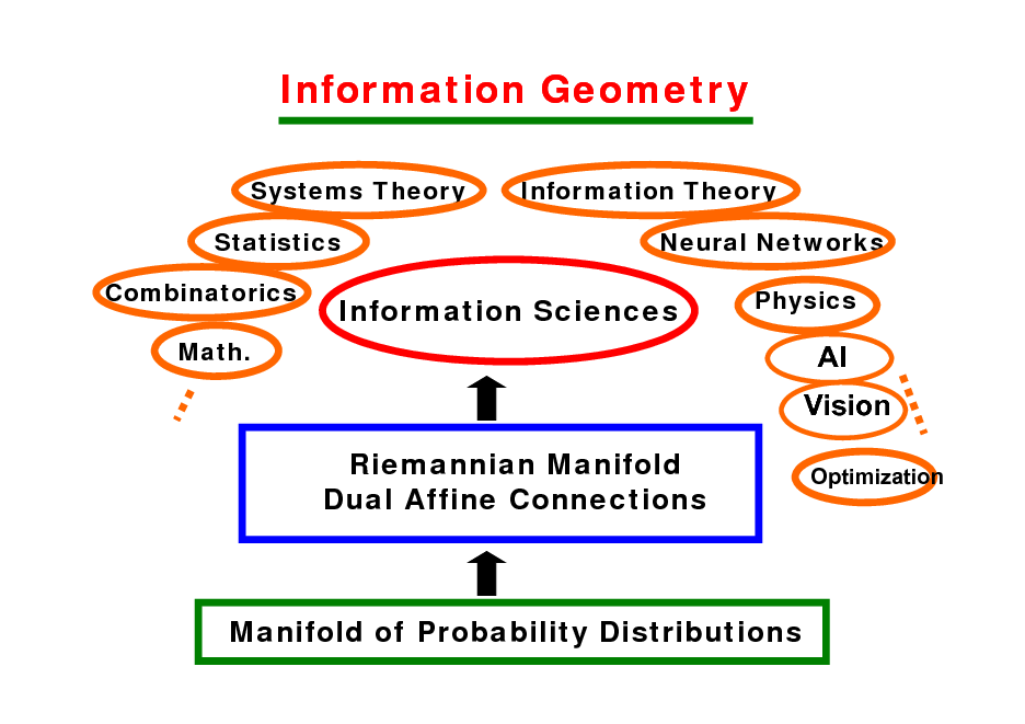
Information Geometry
Systems Theory Statistics Combinatorics Math. Information Theory Neural Networks Physics
Information Sciences
AI Vision Riemannian Manifold Dual Affine Connections
Optimization
Manifold of Probability Distributions
3
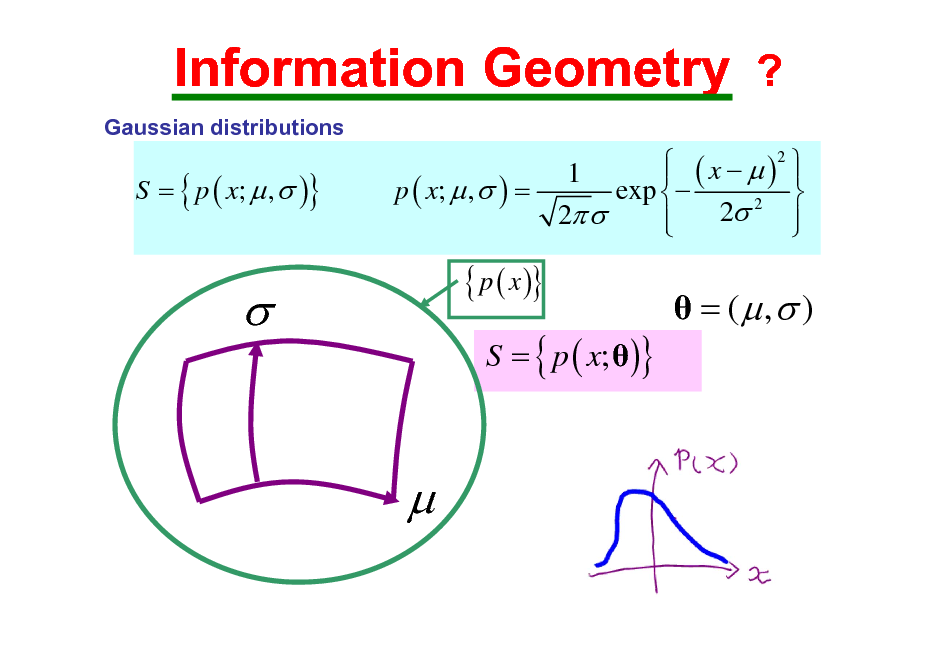
Information Geometry ?
Gaussian distributions
S = { p ( x; , )}
( x )2 1 exp p ( x; , ) = 2 2 2
{ p ( x )}
S = { p ( x; )}
= ( , )
4
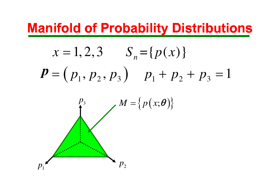
Manifold of Probability Distributions
x = 1, 2, 3
p = ( p1 , p 2 , p3 )
p3
S n ={ p ( x )} p1 + p 2 + p3 = 1
M = { p ( x; )}
p1
p2
5
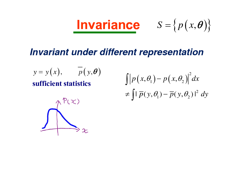
Invariance
S = { p ( x, )}
Invariant under different representation
y = y ( x), p ( y, ) sufficient statistics
p ( x, ) p ( x, ) dx | p ( y, ) p ( y, ) | dy
2 1 2 2 1 2
6
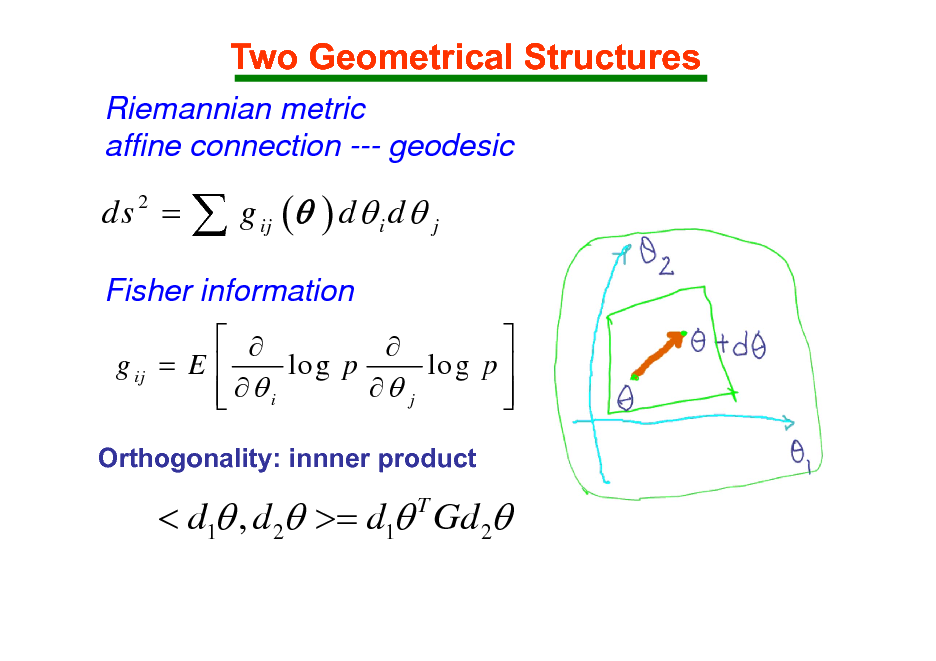
Two Geometrical Structures
Riemannian metric affine connection --- geodesic
ds =
2
g ( ) d d
ij i
j
Fisher information
g ij = E lo g p lo g p j i
Orthogonality: innner product
< d1 , d 2 >= d1 Gd 2
T
7
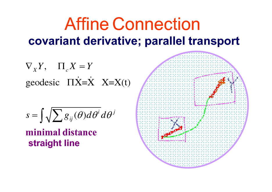
Affine Connection
covariant derivative; parallel transport
XY , c X = Y & & geodesic X=X X=X(t) s= gij ( )d i d j
minimal distance
straight line
8
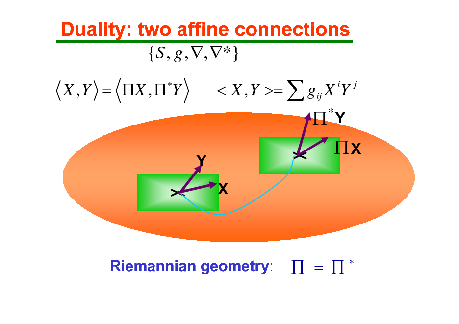
Duality: two affine connections
{S , g , , *}
X , Y = X , Y < X , Y >= gij X iY j
Y X
*
Y
X
Riemannian geometry:
=
9
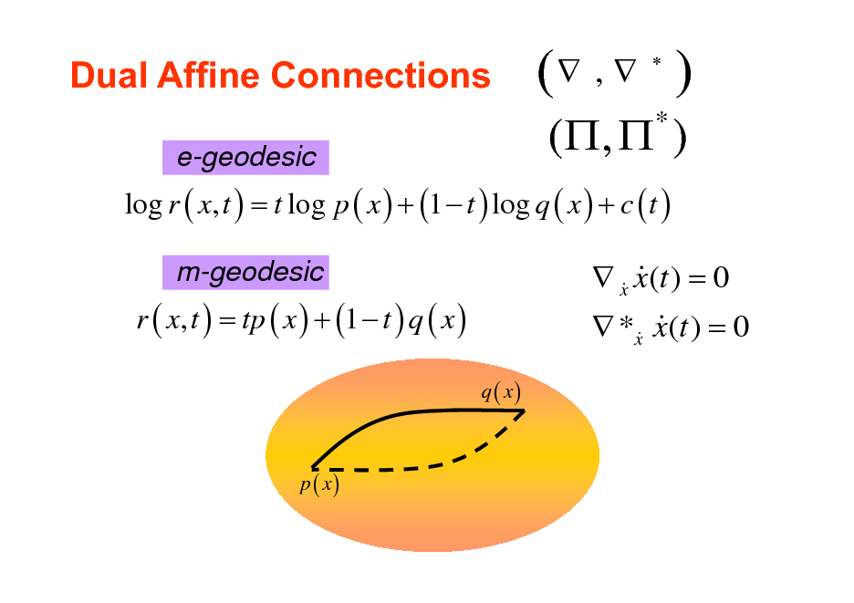
Dual Affine Connections
e-geodesic
( , )
( , )
*
log r ( x, t ) = t log p ( x ) + (1 t ) log q ( x ) + c ( t )
m-geodesic
r ( x, t ) = tp ( x ) + (1 t ) q ( x )
q ( x)
x x(t ) = 0 & & *x x(t ) = 0 & &
p ( x)
10
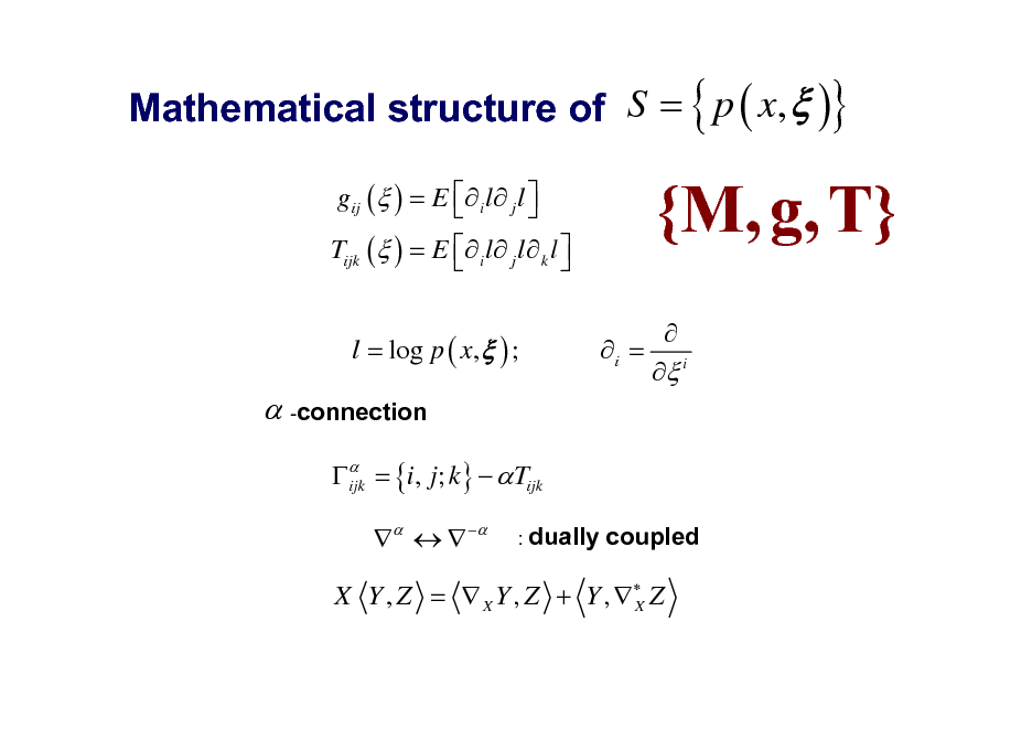
Mathematical structure of S = { p ( x, )}
gij ( ) = E i l j l Tijk ( ) = E i l j l k l
{M, g, T}
i = i
l = log p ( x, ) ;
-connection
= {i, j; k} Tijk ijk
: dually
coupled
X Y , Z = X Y , Z + Y , Z X
11
![Slide: Divergence:
D [ z : y] 0 D [ z : y ] = 0,
D [ z : y]
M
Y Z
iff z = y
D [ z : z + dz ] = gij dzi dz j
positivedefinite](https://yosinski.com/mlss12/media/slides/MLSS-2012-Amari-Information-Geometry_012.png)
Divergence:
D [ z : y] 0 D [ z : y ] = 0,
D [ z : y]
M
Y Z
iff z = y
D [ z : z + dz ] = gij dzi dz j
positivedefinite
12
![Slide: Kullback-Leibler Divergence
quasi-distance
p( x) D[ p ( x) : q ( x)] = p ( x) log q( x) x D[ p ( x) : q ( x)] 0 D[ p : q ] D[q : p ] =0 iff p ( x) = q ( x)](https://yosinski.com/mlss12/media/slides/MLSS-2012-Amari-Information-Geometry_013.png)
Kullback-Leibler Divergence
quasi-distance
p( x) D[ p ( x) : q ( x)] = p ( x) log q( x) x D[ p ( x) : q ( x)] 0 D[ p : q ] D[q : p ] =0 iff p ( x) = q ( x)
13
![Slide: % f divergence of S
% % S = { p} , % % pi > 0 : ( pi = 1 nn holds)
0 qi % % % % D f [ p : q ] = pi f % pi
% % % % D f [ p : q] = 0 p = q
% not invariant under f ( u ) = f ( u ) c ( u 1)](https://yosinski.com/mlss12/media/slides/MLSS-2012-Amari-Information-Geometry_014.png)
% f divergence of S
% % S = { p} , % % pi > 0 : ( pi = 1 nn holds)
0 qi % % % % D f [ p : q ] = pi f % pi
% % % % D f [ p : q] = 0 p = q
% not invariant under f ( u ) = f ( u ) c ( u 1)
14
![Slide: divergence
1 1+ % % % % % D [ p : q ] = { pi + qi pi 2 2
1 2
% qi
1+ 2
}
KL-divergence
% pi % % % % % D[ p : q ] = { pi log + pi qi } % qi](https://yosinski.com/mlss12/media/slides/MLSS-2012-Amari-Information-Geometry_015.png)
divergence
1 1+ % % % % % D [ p : q ] = { pi + qi pi 2 2
1 2
% qi
1+ 2
}
KL-divergence
% pi % % % % % D[ p : q ] = { pi log + pi qi } % qi
15
![Slide: ( , ) divergence
D , [ p : q] = {
+
pi
+
+
+
qi + p i qi }
= : divergence = 1: -divergence](https://yosinski.com/mlss12/media/slides/MLSS-2012-Amari-Information-Geometry_016.png)
( , ) divergence
D , [ p : q] = {
+
pi
+
+
+
qi + p i qi }
= : divergence = 1: -divergence
16
![Slide: MetricandConnectionsInducedbyDivergence Riemannian metric
(Eguchi)
1 gij ( z ) = i j D [ z : y ] y= z : D [ z : z + dz ] = gij ( z ) dzi dz j 2
affine connections
ijk ( z ) = i j 'k D [ z : y ] y= z
ijk
{, *} i = , zi = yi
' i
( z ) = j k D [ z : y] y= z
' i '](https://yosinski.com/mlss12/media/slides/MLSS-2012-Amari-Information-Geometry_017.png)
MetricandConnectionsInducedbyDivergence Riemannian metric
(Eguchi)
1 gij ( z ) = i j D [ z : y ] y= z : D [ z : z + dz ] = gij ( z ) dzi dz j 2
affine connections
ijk ( z ) = i j 'k D [ z : y ] y= z
ijk
{, *} i = , zi = yi
' i
( z ) = j k D [ z : y] y= z
' i '
17
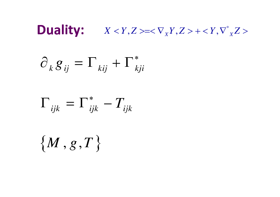
Duality:
X < Y , Z >=< X Y , Z > + < Y , * X Z >
kji
k g ij = kij + ijk =
ijk
Tijk
{M , g , T }
18
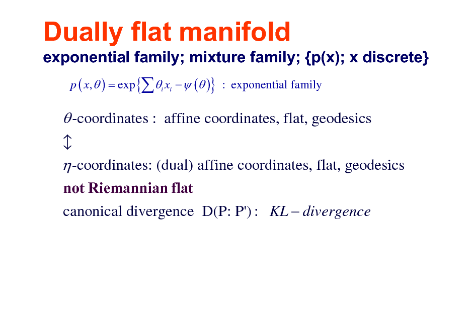
Dually flat manifold
exponential family; mixture family; {p(x); x discrete}
p ( x, ) = exp { i xi ( )} : exponential family
-coordinates : affine coordinates, flat, geodesics -coordinates: (dual) affine coordinates, flat, geodesics
not Riemannian flat canonical divergence D(P: P') : KL divergence b
19
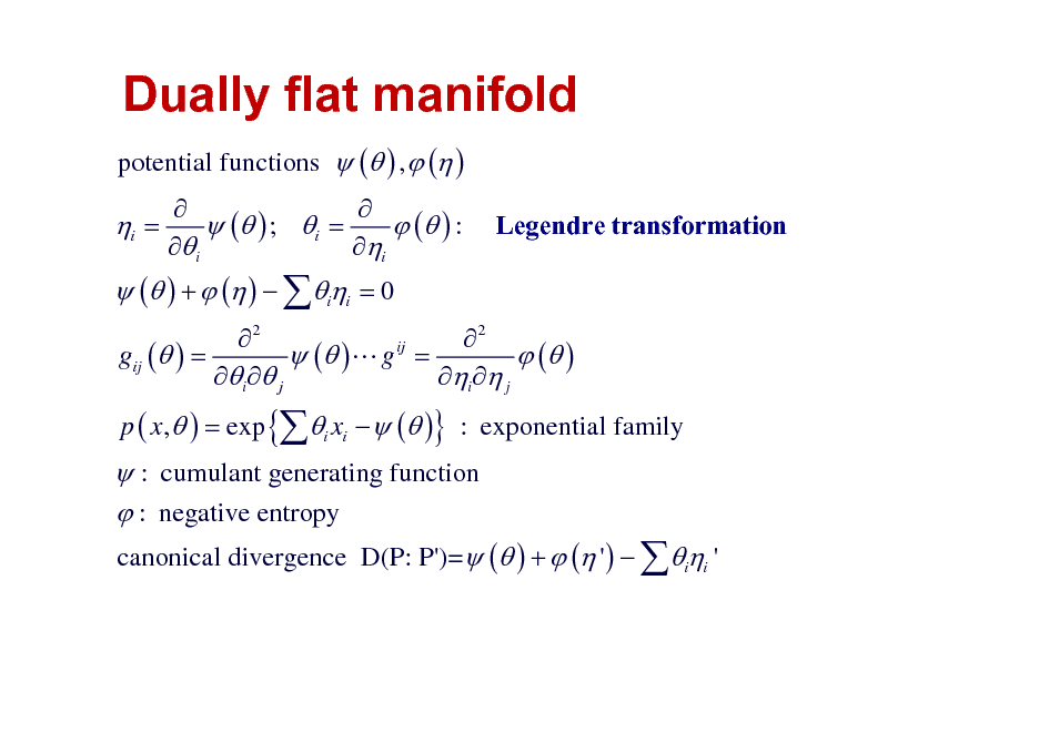
Dually flat manifold
potential functions ( ) , ( )
i =
( ) + ( ) ii = 0
( ) ; i = ( ) : i i
Legendre transformation
2 2 ij gij ( ) = ( )L g = ( ) i j i j p ( x, ) = exp {i xi ( )} : exponential family
: cumulant generating function : negative entropy
canonical divergence D(P: P')= ( ) + ( ' ) ii '
20
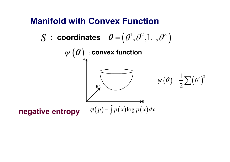
Manifold with Convex Function
S
: coordinates
( )
= ( 1 , 2 ,L , n )
function
: convex
1 i 2 ( ) = ( ) 2
( p ) = p ( x ) log p ( x ) dx
negative entropy
21
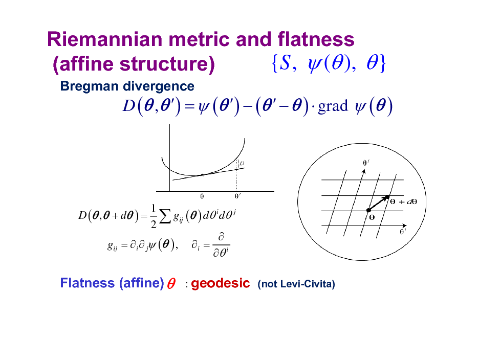
Riemannian metric and flatness {S , ( ), } (affine structure)
Bregman divergence
D ( , ) = ( ) ( ) grad ( )
D ( , + d ) =
1 gij ( ) d i d j 2 gij = i j ( ) , i = i
: geodesic (not Levi-Civita)
Flatness (affine)
22
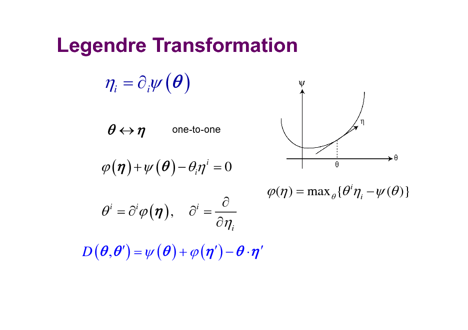
Legendre Transformation
i = i ( )
one-to-one
( ) + ( ) i i = 0
= ( ) ,
i i
= i
i
( ) = max { ii ( )}
D ( , ) = ( ) + ( )
23
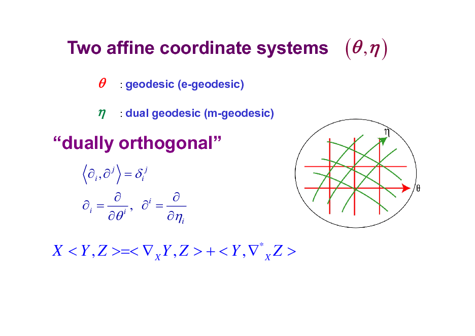
Two affine coordinate systems
: geodesic (e-geodesic) : dual geodesic (m-geodesic)
( , )
dually orthogonal
i , j = i j i = , i = i i
X < Y , Z >=< X Y , Z > + < Y , * X Z >
24
![Slide: Pythagorean Theorem
(dually flat manifold)
D [ P : Q ] + D [Q : R ] = D [ P : R ]
Euclidean space: self-dual
( ) =
1 2 (i ) 2
=](https://yosinski.com/mlss12/media/slides/MLSS-2012-Amari-Information-Geometry_025.png)
Pythagorean Theorem
(dually flat manifold)
D [ P : Q ] + D [Q : R ] = D [ P : R ]
Euclidean space: self-dual
( ) =
1 2 (i ) 2
=
25
![Slide: Projection Theorem
min D [ P : Q ]
QM
Q = m-geodesic projection of P to M
min D [Q : P ]
QM
Q = e-geodesic projection of P to M](https://yosinski.com/mlss12/media/slides/MLSS-2012-Amari-Information-Geometry_026.png)
Projection Theorem
min D [ P : Q ]
QM
Q = m-geodesic projection of P to M
min D [Q : P ]
QM
Q = e-geodesic projection of P to M
26
![Slide: Two Types of Divergence
Invariant divergence (Chentsov, Csiszar) f-divergence: Fisher- structure
D [p : q] =
p(x)f{
q(x) }dx p(x)
Flat divergence (Bregman) convex function
KL-divergence belongs to both classes: flat and invariant](https://yosinski.com/mlss12/media/slides/MLSS-2012-Amari-Information-Geometry_027.png)
Two Types of Divergence
Invariant divergence (Chentsov, Csiszar) f-divergence: Fisher- structure
D [p : q] =
p(x)f{
q(x) }dx p(x)
Flat divergence (Bregman) convex function
KL-divergence belongs to both classes: flat and invariant
27
![Slide: divergence
S = {p} : space of probability distributions
invariance
invariantdivergence
F-divergence Fisher inf metric Alpha connection
duallyflatspace
Flatdivergence
convexfunctions Bregman
KLdivergence
p(x) D[p : q] = p(x) log{ }dx q(x)](https://yosinski.com/mlss12/media/slides/MLSS-2012-Amari-Information-Geometry_028.png)
divergence
S = {p} : space of probability distributions
invariance
invariantdivergence
F-divergence Fisher inf metric Alpha connection
duallyflatspace
Flatdivergence
convexfunctions Bregman
KLdivergence
p(x) D[p : q] = p(x) log{ }dx q(x)
28
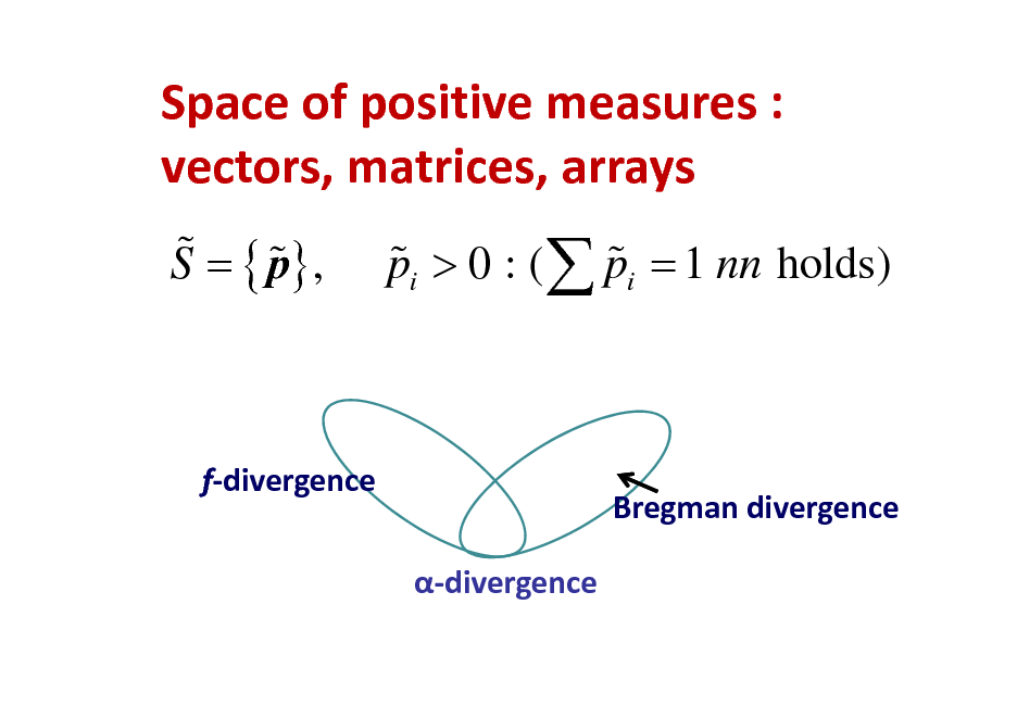
Spaceofpositivemeasures: vectors,matrices,arrays
% % S = { p} , % % pi > 0 : ( pi = 1 nn holds)
fdivergence divergence
Bregmandivergence
29
Applications of Information Geometry
Statistical Inference Machine Learning and AI Computer Vision Convex Programming Signal Processing (ICA; Sparse) Information Theory, Systems Theory Quantum Information Geometry
30
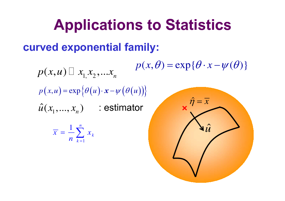
Applications to Statistics
curved exponential family:
p ( x, u )
x1, x2 ,...xn
p ( x, ) = exp{ x ( )}
p ( x, u ) = exp ( u ) x ( ( u ) )
{
}
u ( x1 ,..., xn )
1 x = n
: estimator
xk
=x
n
u
k =1
31
![Slide: x : discrete
X = {0, 1, , n}
S n = { p ( x) | x X }:
n i =0
exponential family
n i i =1
p ( x) = pi i ( x) = exp[ xi ( )]
= log pi log p0 ; xi = i ( x); ( ) = log p0
i
statistical model : p ( x, u )](https://yosinski.com/mlss12/media/slides/MLSS-2012-Amari-Information-Geometry_032.png)
x : discrete
X = {0, 1, , n}
S n = { p ( x) | x X }:
n i =0
exponential family
n i i =1
p ( x) = pi i ( x) = exp[ xi ( )]
= log pi log p0 ; xi = i ( x); ( ) = log p0
i
statistical model : p ( x, u )
32
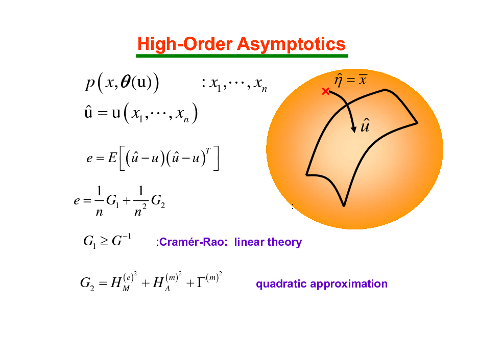
High-Order Asymptotics
p ( x, (u) ) u = u ( x1 ,L , xn ) : x1 ,L , xn
=x
u
( u u )( u u )T e=E
1 1 e = G1 + 2 G2 n n
:
G1 G 1
( e )2
:Cramr-Rao: linear theory
( m )2
G2 = H M + H A
+
( m )2
quadratic approximation
33

Information Geometry of Belief Propagation
Shun-ichi Amari (RIKEN BSI) Shiro Ikeda (Inst. Statist. Math.) Toshiyuki Tanaka (Kyoto U.)
34
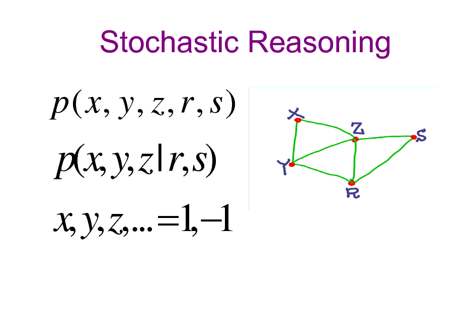
Stochastic Reasoning
p ( x, y , z , r , s )
p(x, y, z | r, s) x, y, z,... =1 1 ,
35
![Slide: Stochastic Reasoning
q(x1,x2,x3,| observation) X= (x1 x2 x3 ..) x = 1, -1 maximum likelihood
= argmax q(x1, x2 ,x3 ,..) i = sgn E[xi]
least bit error rate estimator](https://yosinski.com/mlss12/media/slides/MLSS-2012-Amari-Information-Geometry_036.png)
Stochastic Reasoning
q(x1,x2,x3,| observation) X= (x1 x2 x3 ..) x = 1, -1 maximum likelihood
= argmax q(x1, x2 ,x3 ,..) i = sgn E[xi]
least bit error rate estimator
36
![Slide: Mean Value
Marginalization: projection to independent distributions
0 q (x) = q1 ( x1 )q2 ( x2 )...qn ( xn ) = q0 (x)
( q i ( x i ) = q ( x1, ..., x n ) d x1 ..d x i ..d x n
= E [ x] = E
q
q0
[ x]](https://yosinski.com/mlss12/media/slides/MLSS-2012-Amari-Information-Geometry_037.png)
Mean Value
Marginalization: projection to independent distributions
0 q (x) = q1 ( x1 )q2 ( x2 )...qn ( xn ) = q0 (x)
( q i ( x i ) = q ( x1, ..., x n ) d x1 ..d x i ..d x n
= E [ x] = E
q
q0
[ x]
37
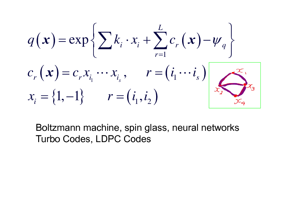
q ( x ) = exp ki xi + cr ( x ) q r =1 cr ( x ) = cr xi1 L xis , r = ( i1 L is )
L
q Boltzmann p { wijspin jglass, neural } ( x ) = ex machine, xi x + hi xi networks
Turbo Codes, LDPC Codes
xi = {1, 1}
r = ( i1 , i2 )
38
![Slide: Computationally Difficult
q ( x ) = E [ x]
q ( x ) = exp { cr ( x ) q }
mean-field approximation belief propagation tree propagation, CCCP (convex-concave)](https://yosinski.com/mlss12/media/slides/MLSS-2012-Amari-Information-Geometry_039.png)
Computationally Difficult
q ( x ) = E [ x]
q ( x ) = exp { cr ( x ) q }
mean-field approximation belief propagation tree propagation, CCCP (convex-concave)
39
![Slide: Information Geometry of Mean Field Approximation
m-projection e-projection D[q:p]=
m 0
q(x) q(x)log p(x) x
q = argmin D[q:p]
e q 0
= argmin D[p:q]
p( x ) M 0
M0 = {i pi ( xi )}](https://yosinski.com/mlss12/media/slides/MLSS-2012-Amari-Information-Geometry_040.png)
Information Geometry of Mean Field Approximation
m-projection e-projection D[q:p]=
m 0
q(x) q(x)log p(x) x
q = argmin D[q:p]
e q 0
= argmin D[p:q]
p( x ) M 0
M0 = {i pi ( xi )}
40
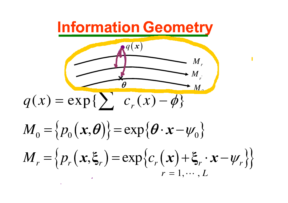
Information Geometry
q( x)
Mr
M r' M0
q ( x ) = exp{ cr ( x ) }
M0 = { p0 ( x, )} = exp{ x 0}
M r = pr ( x, r ) = exp{cr ( x ) + r x r }
r = 1, L , L
{
}
41
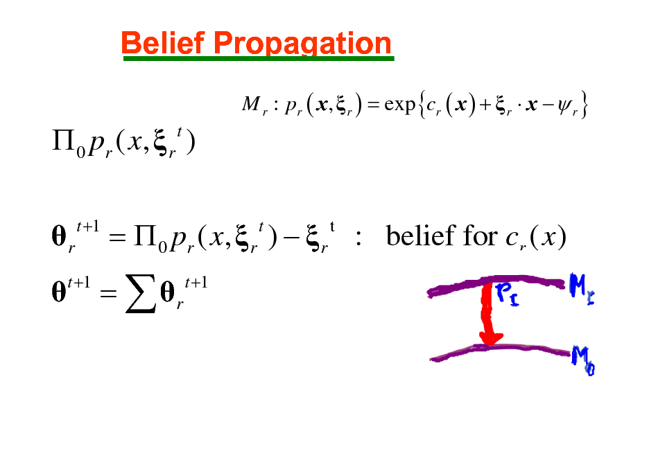
Belief Propagation
M r : pr ( x , r ) = exp {cr ( x ) + r x r }
0 pr ( x , r )
t
r
t +1
= 0 pr ( x, r ) r : belief for cr ( x )
t t t +1
t +1
= r
42
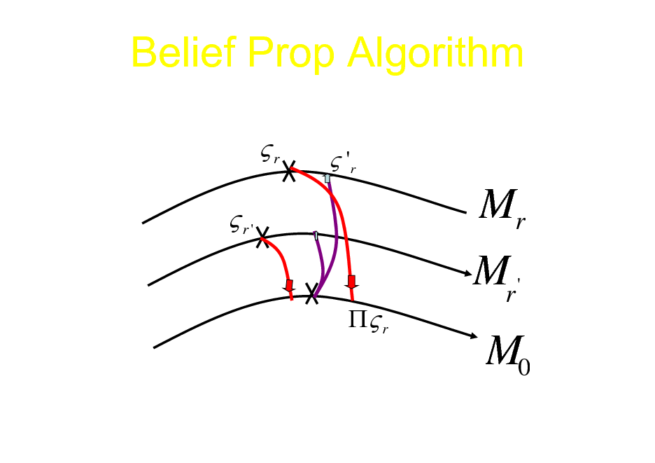
Belief Prop Algorithm
r r'
r
'r
Mr
Mr '
M0
43
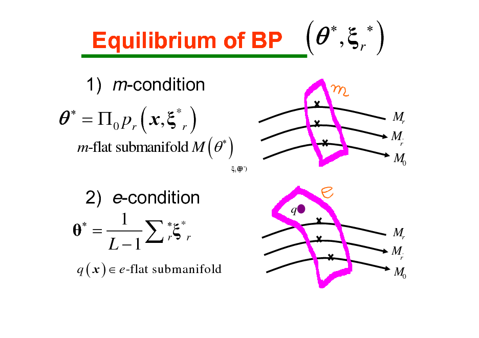
Equilibrium of BP
1) m-condition
(
, r
)
Mr
= 0 pr ( x , * r )
m-flat submanifold M (
)
1 ( ')
Mr' M0
2) e-condition 1 * = r r L 1
q ( x ) e -flat submanifold
q
Mr
Mr'
M0
44
![Slide: Free energy:
F(,1,L,L ) = D[ p0 : q] D[ p0 : pr ]
critical point
F =0 F =0 r
not convex
: e-condition : m-condition](https://yosinski.com/mlss12/media/slides/MLSS-2012-Amari-Information-Geometry_045.png)
Free energy:
F(,1,L,L ) = D[ p0 : q] D[ p0 : pr ]
critical point
F =0 F =0 r
not convex
: e-condition : m-condition
45
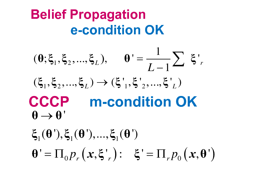
Belief Propagation e-condition OK
1 ( ; 1 , 2 ,..., L ), ' = 'r L 1 ( 1 , 2 ,..., L ) ( '1 , ' 2 ,..., ' L )
CCCP
'
m-condition OK
1 ( '), 1 ( '),..., 1 ( ')
' = 0 pr ( x, ' r ) : ' = r p0 ( x, ' )
46
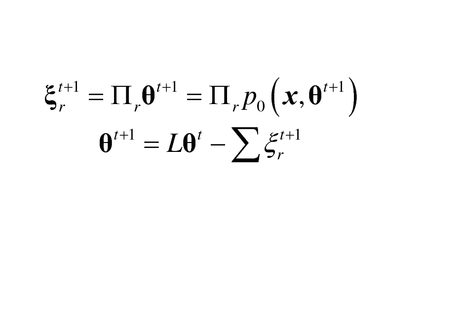
t +1 r
= r
t +1
t +1
= L
t
= r p0 ( x,
t +1 r
t +1
)
47
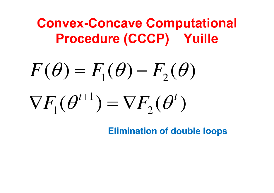
Convex-Concave Computational Procedure (CCCP) Yuille
F ( ) = F1 ( ) F2 ( ) F1 (
t +1
) = F2 ( )
t
Elimination of double loops
48
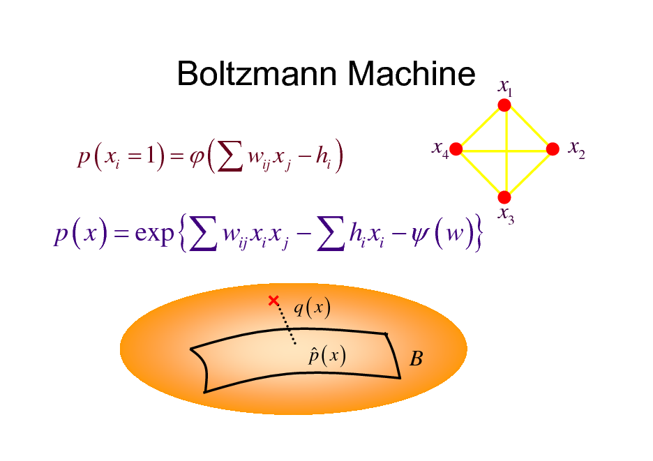
Boltzmann Machine
p ( xi = 1) = ( wij x j hi )
x4
x1 x2
x3
p ( x ) = exp { wij xi x j hi xi ( w )}
q ( x) p ( x)
B
49
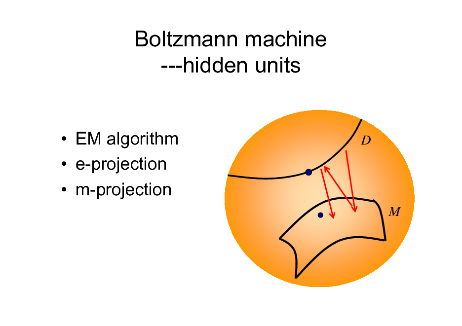
Boltzmann machine ---hidden units
EM algorithm e-projection m-projection
D
M
50
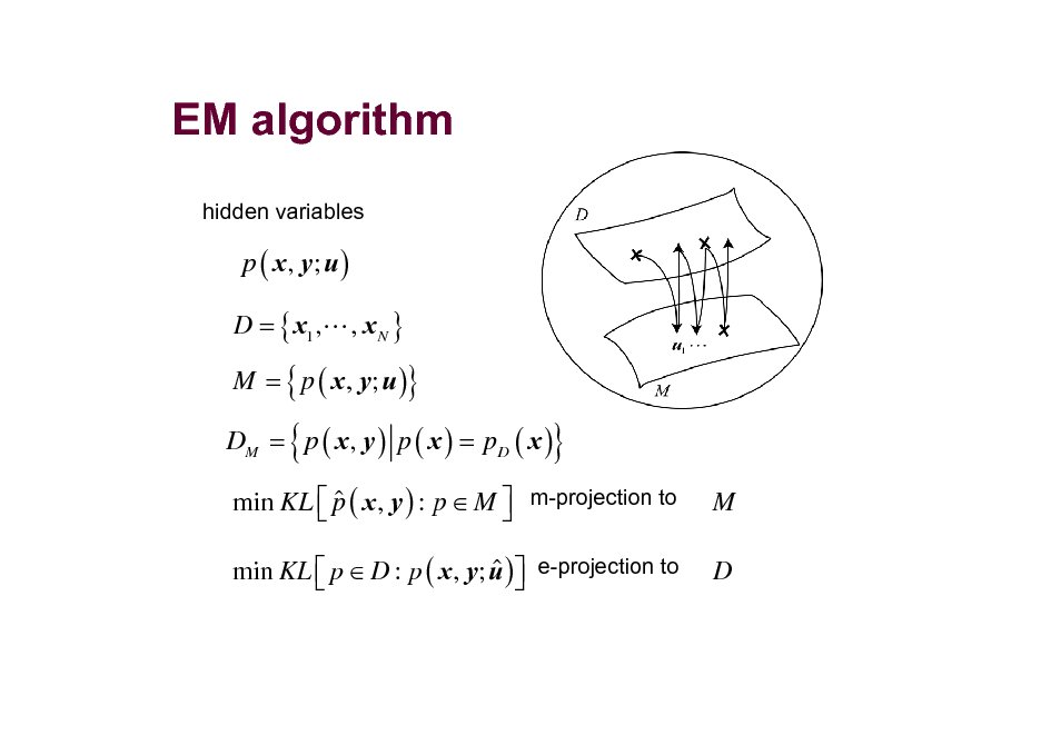
EM algorithm
hidden variables
p ( x , y; u ) D = { x1 ,L , x N } M = { p ( x , y; u )}
DM = p ( x , y ) p ( x ) = pD ( x )
{
}
M D
min KL p ( x , y ) : p M m-projection to
min KL p D : p ( x , y; u ) e-projection to
51
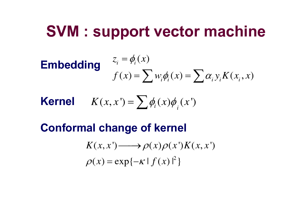
SVM : support vector machine
Embedding Kernel
zi = i ( x) f ( x) = wii ( x) = i yi K ( xi , x)
K ( x, x ') = i ( x) i ( x ')
K ( x, x ') ( x ) ( x ') K ( x, x ')
Conformal change of kernel
( x ) = exp{ | f ( x ) |2 }
52
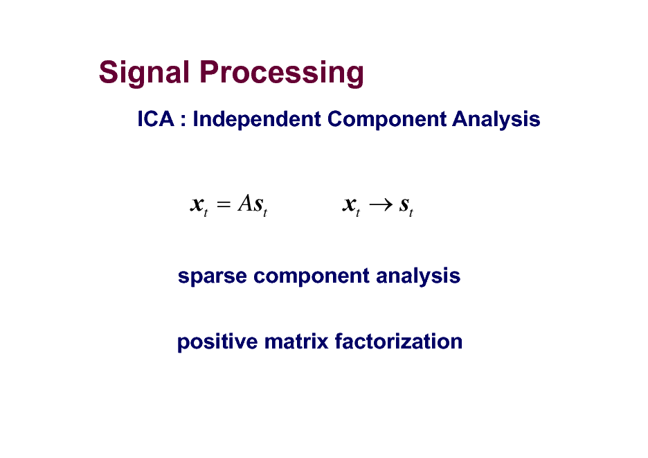
Signal Processing
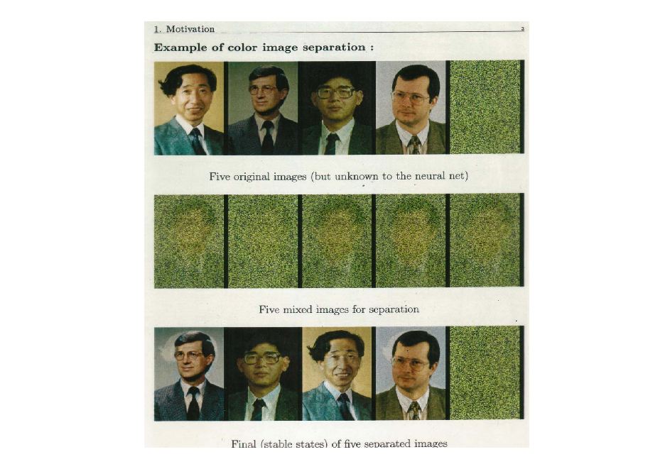
ICA : Independent Component Analysis
xt = Ast
xt st
sparse component analysis positive matrix factorization
53
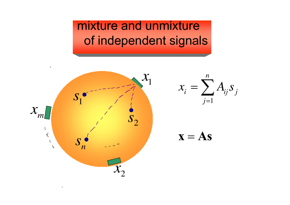
mixture and unmixture of independent signals
x1
xm
s1 s2 sn x2
xi = Aij s j
j =1
n
x = As
54
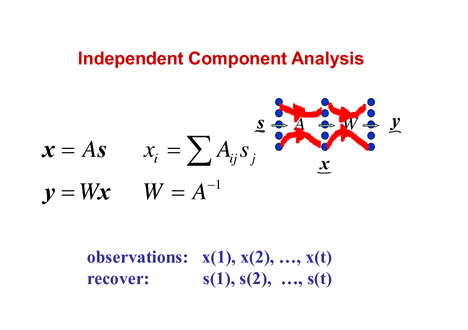
Independent Component Analysis
x = As y = Wx
xi = Aij s j W=A
1
s
A
W
y
x
observations: x(1), x(2), , x(t) recover: s(1), s(2), , s(t)
55
56
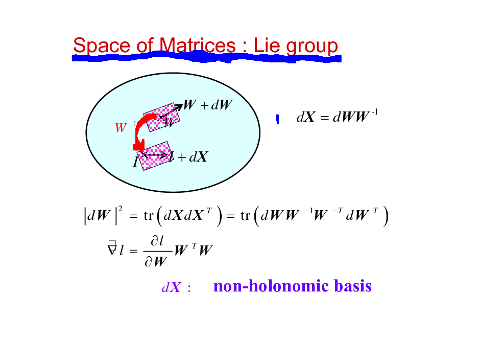
Space of Matrices : Lie group
W + dW
W 1
W
dX = dWW -1
I
dW
2
I + dX
= tr ( d X d X T
) = tr ( d W W
1
W
T
dW
T
)
l W TW l = W
dX :
non-holonomic basis
57
![Slide: Information Geometry of ICA
S ={p(y)}
r
q
I = {q1 ( y1 )q2 ( y2 )...qn ( yn )}
{ p (Wx)}
natural gradient l ( W) = KL[ p (y; W) : q (y )] estimating function r (y ) stability, efficiency](https://yosinski.com/mlss12/media/slides/MLSS-2012-Amari-Information-Geometry_058.png)
Information Geometry of ICA
S ={p(y)}
r
q
I = {q1 ( y1 )q2 ( y2 )...qn ( yn )}
{ p (Wx)}
natural gradient l ( W) = KL[ p (y; W) : q (y )] estimating function r (y ) stability, efficiency
58
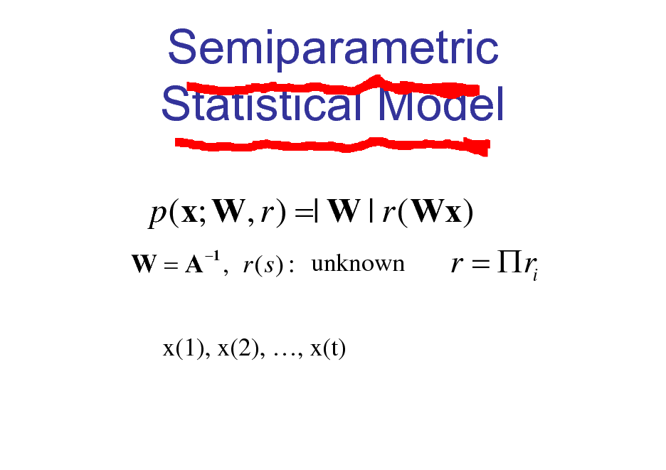
Semiparametric Statistical Model
p (x; W, r ) =| W | r ( Wx) 1 r = ri W = A , r ( s ) : unknown
x(1), x(2), , x(t)
59
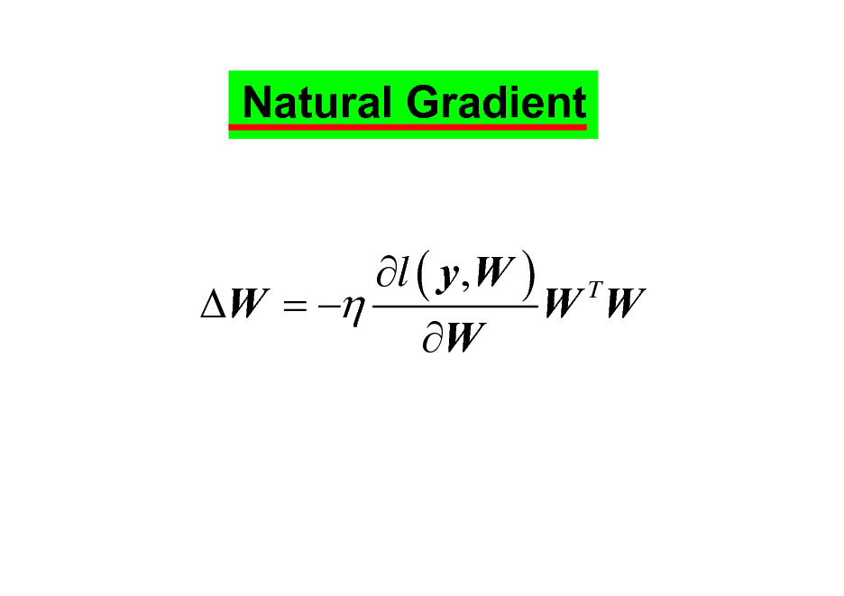
Natural Gradient
l ( y, W ) T W = W W W
60
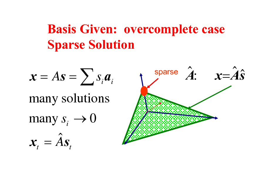
Basis Given: overcomplete case Sparse Solution
x = As = si ai many solutions many si 0 x = As
t t
sparse
A:
x = As
61
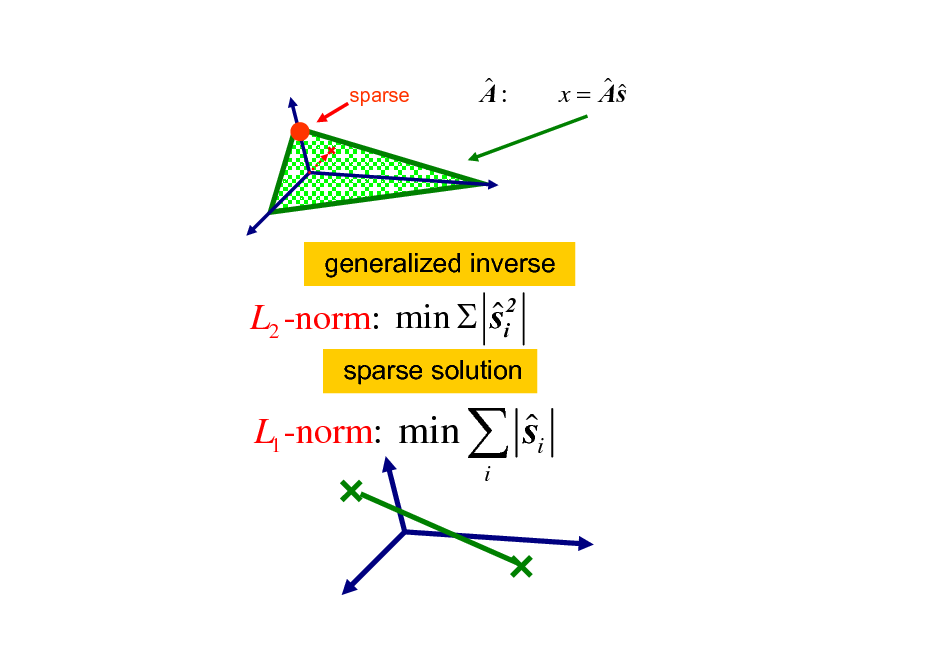
sparse
A:
x = As
generalized inverse
min si2 L2 -norm:
sparse solution
L1 -norm: min
s
i
i
62
63
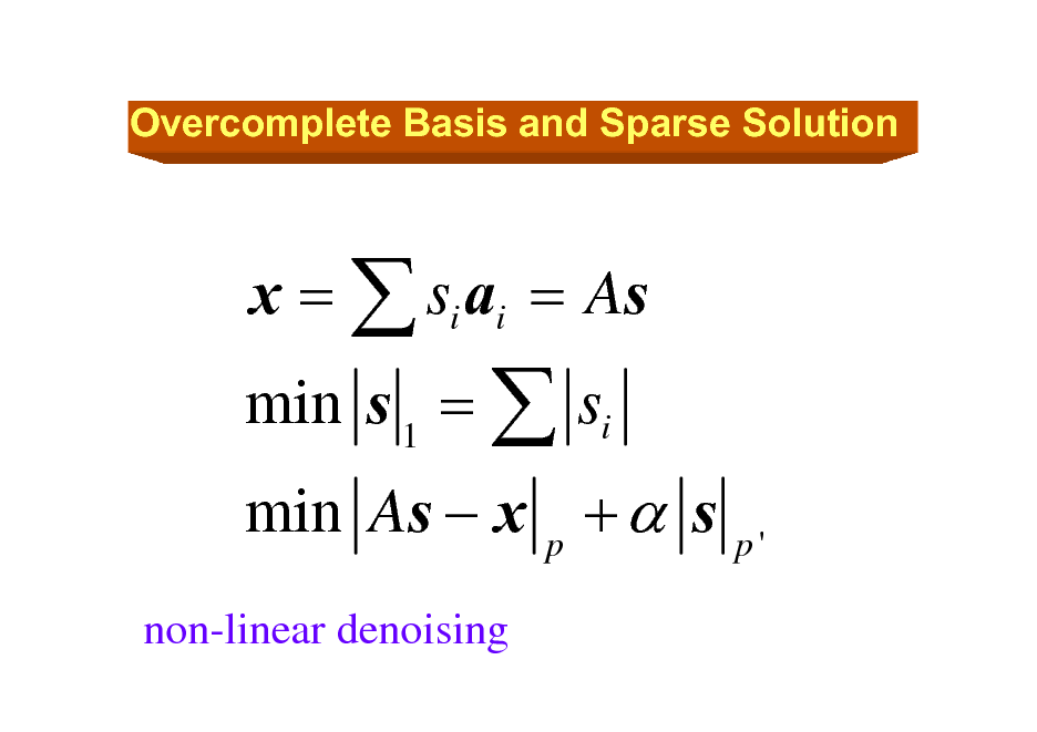
Overcomplete Basis and Sparse Solution
min s 1 = si
non-linear denoising
x = si ai = As
min As x p + s
p'
64
![Slide: Sparse Solution
min ( ) penalty Fp ( ) = i
F0 ( ) = #1[ i 0] : sparsest solution F1 ( ) = i : L1 solution Fp ( ) : 0 p 1
2
p
: Bayes prior
Sparse solution: overcomplete case
F2 ( ) = i : generalized inverse solution](https://yosinski.com/mlss12/media/slides/MLSS-2012-Amari-Information-Geometry_065.png)
Sparse Solution
min ( ) penalty Fp ( ) = i
F0 ( ) = #1[ i 0] : sparsest solution F1 ( ) = i : L1 solution Fp ( ) : 0 p 1
2
p
: Bayes prior
Sparse solution: overcomplete case
F2 ( ) = i : generalized inverse solution
65
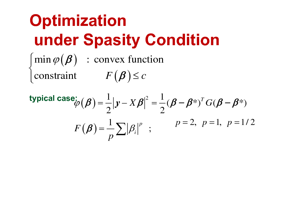
Optimization under Spasity Condition
min ( ) : convex function F ( ) c constraint
typical case:
1 1 2 ( ) = y X = ( *)T G ( *) 2 2 p = 2, p = 1, p = 1/ 2 p 1 F ( ) = i ; p
66
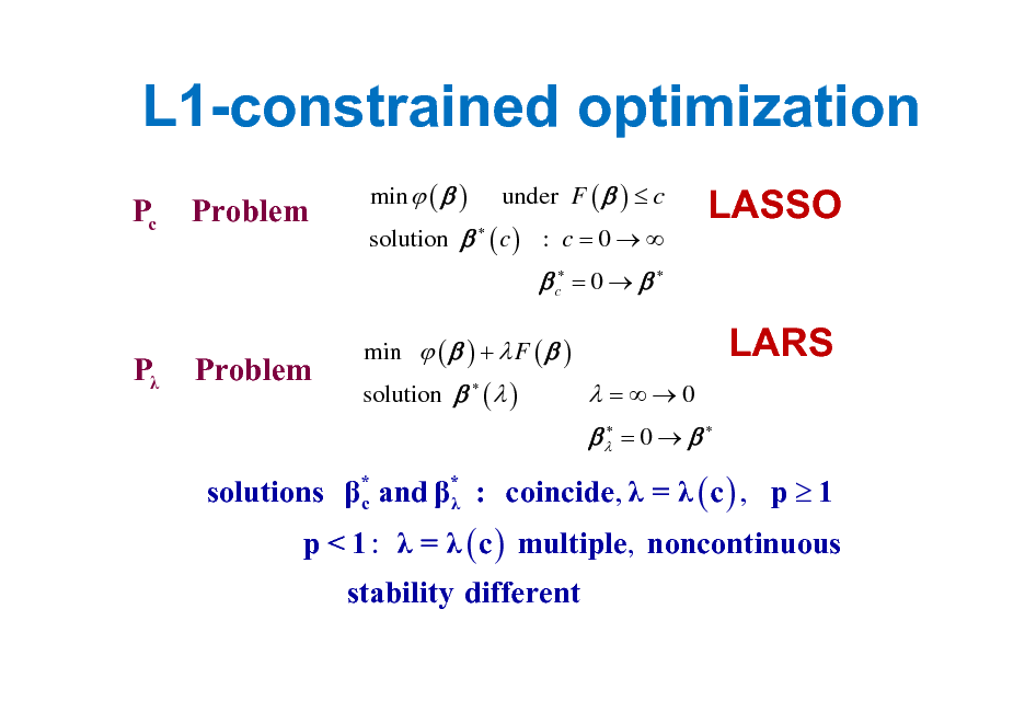
L1-constrained optimization
Pc Problem
min ( ) under F ( ) c solution ( c ) : c = 0
LASSO LARS
c = 0
P Problem
min ( ) + F ( ) solution ( )
=0
= 0
solutions * and * : coincide, = ( c ) , p 1 c p < 1 : = ( c ) multiple, noncontinuous stability different
67
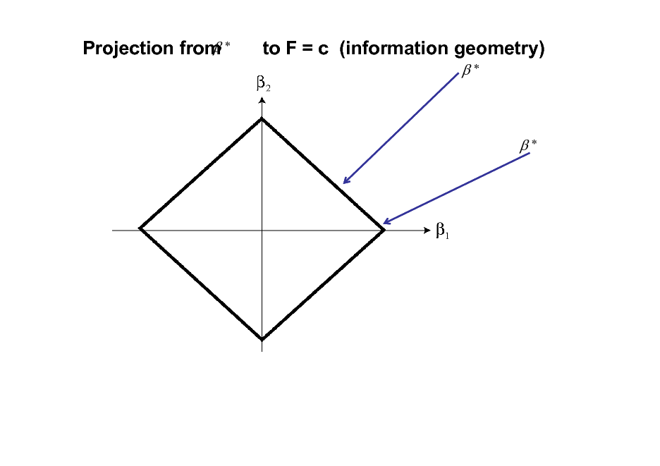
Projection from *
to F = c (information geometry)
*
*
68
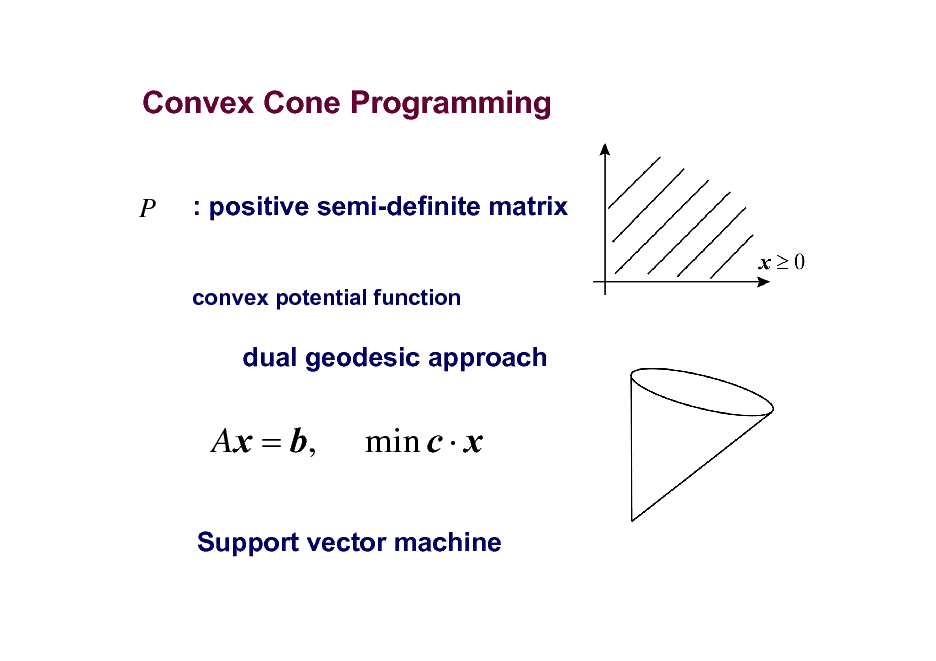
Convex Cone Programming
: positive semi-definite matrix
convex potential function
P
dual geodesic approach
Ax = b,
min c x
Support vector machine
69
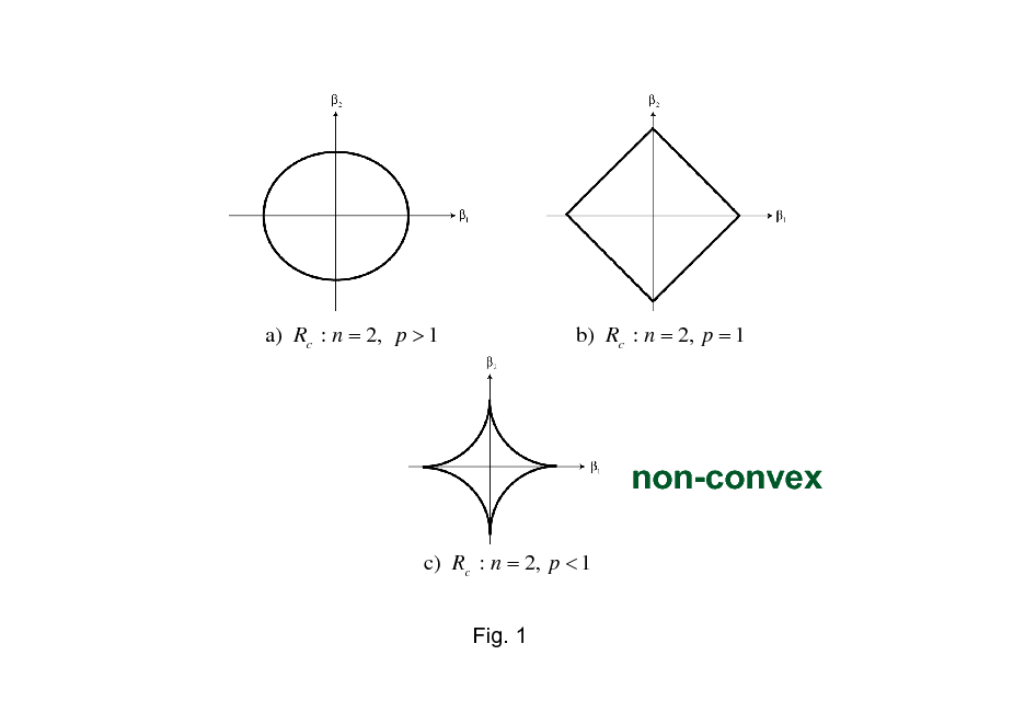
a) Rc : n = 2, p > 1
b) Rc : n = 2, p = 1
non-convex
c) Rc : n = 2, p < 1 Fig. 1
70
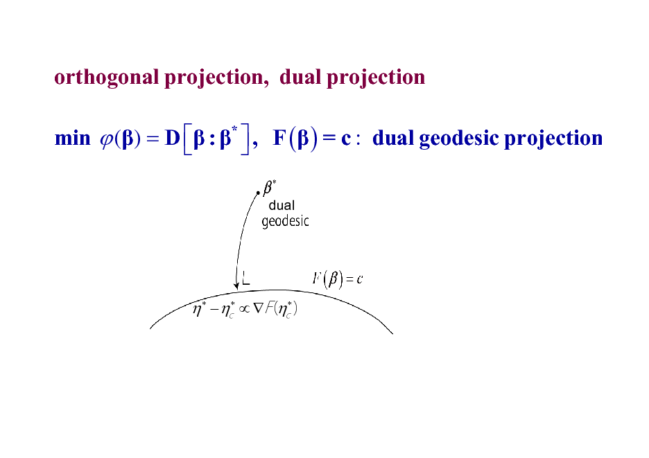
orthogonal projection, dual projection min () = D : * , F ( ) = c : dual geodesic projection
dual
71
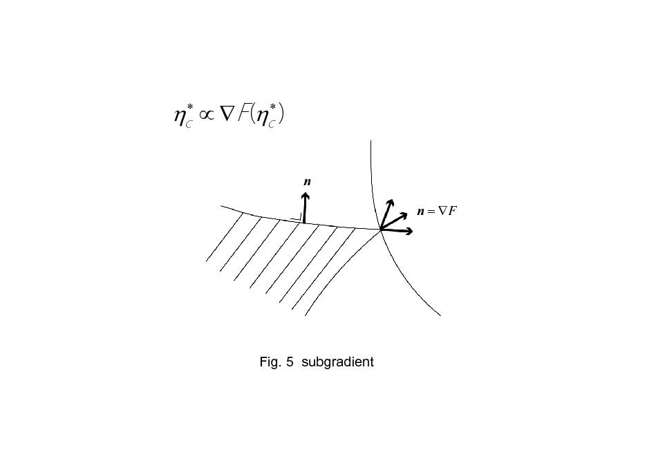
n n = F
Fig. 5 subgradient
72
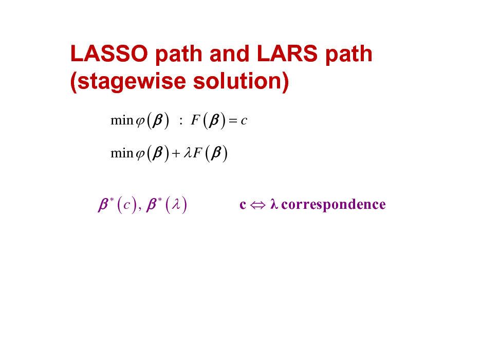
LASSO path and LARS path (stagewise solution)
min ( ) : F ( ) = c min ( ) + F ( )
(c) , ( )
c correspondence
73
![Slide: Active set and gradient
A ( ) = {i i 0} sgn ( i ) i (1 p ) , i A Fp ( ) = ( , ) , i A [ 1,1]](https://yosinski.com/mlss12/media/slides/MLSS-2012-Amari-Information-Geometry_074.png)
Active set and gradient
A ( ) = {i i 0} sgn ( i ) i (1 p ) , i A Fp ( ) = ( , ) , i A [ 1,1]
74
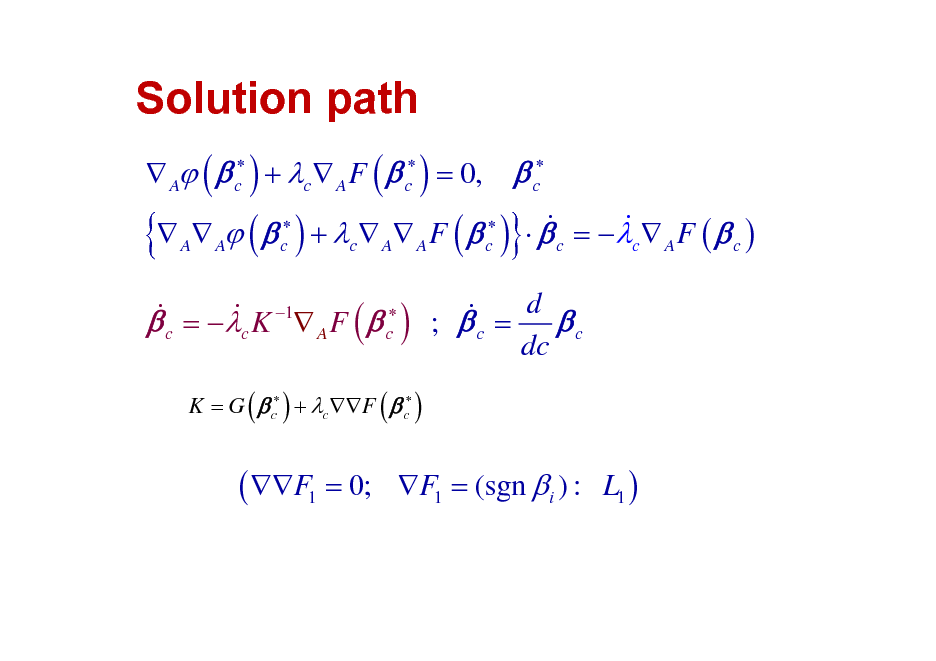
Solution path
{
A ( c ) + c A F ( c ) = 0,
c
& & A A ( c ) + c A A F ( c ) c = c A F ( c )
}
& = K 1 F ( ) ; = d & & c A c c c c dc
K = G ( c ) + cF ( c )
( F1 = 0;
F1 = (sgn i ) : L1 )
75
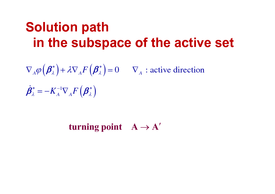
Solution path in the subspace of the active set
A ( ) + A F ( ) = 0 & = K A1 A F ( )
A : active direction
turning point A A
76
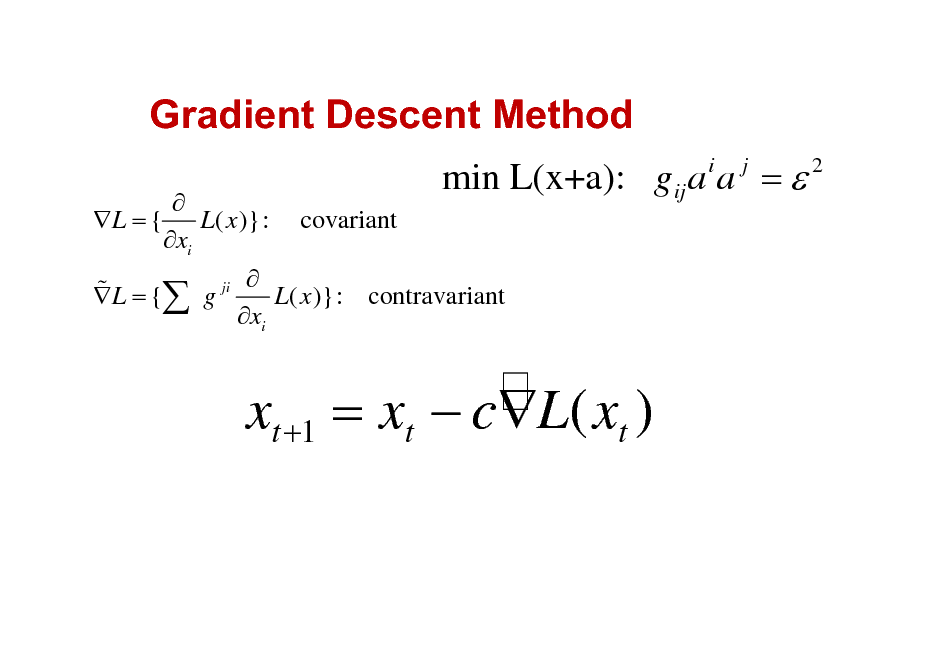
Gradient Descent Method
L = { L( x )}: xi
min L(x+a): gij a a =
i j
2
covariant
ji %L ={ g x L( x )}: contravariant i
xt +1 = xt cL( xt )
77
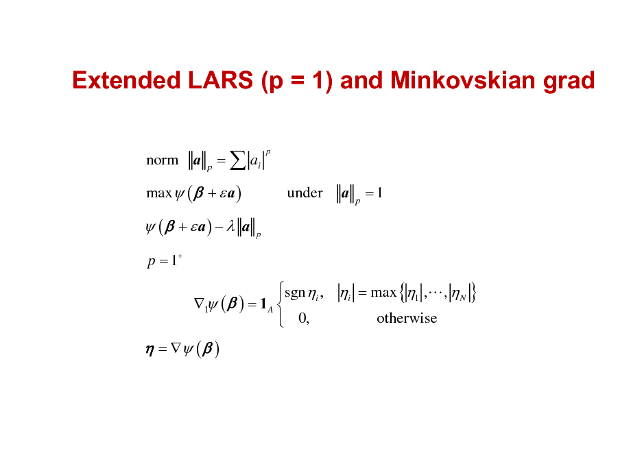
Extended LARS (p = 1) and Minkovskian grad
norm a = ai
p
p
max ( + a )
under
p
a
p
=1
( + a) a
p = 1+
sgni , i = max {1 ,L , N } 1 ( ) = 1 A otherwise 0,
= ( )
78
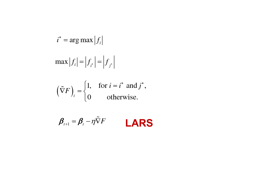
i = arg max fi
max fi = fi = f j
% ( F )
i
1, for i = i and j , = otherwise. 0
% t +1 = t F
LARS
79
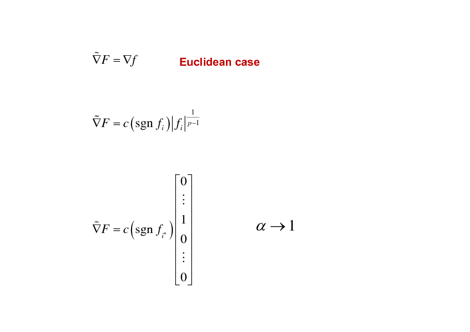
% F = f
Euclidean case
% F = c ( sgn fi ) fi
1 p 1
% F = c sgn fi
(
)
0 M 1 0 M 0
1
80
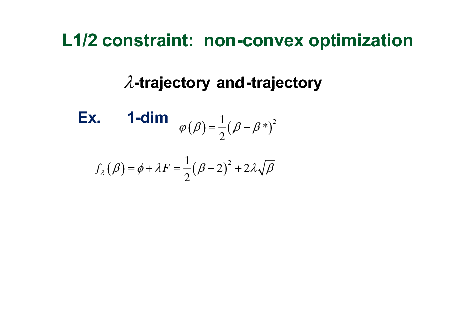
L1/2 constraint: non-convex optimization
-trajectory
Ex. 1-dim
( ) =
and-trajectory c
1 2 *) ( 2
1 2 f ( ) = + F = ( 2 ) + 2 2
81
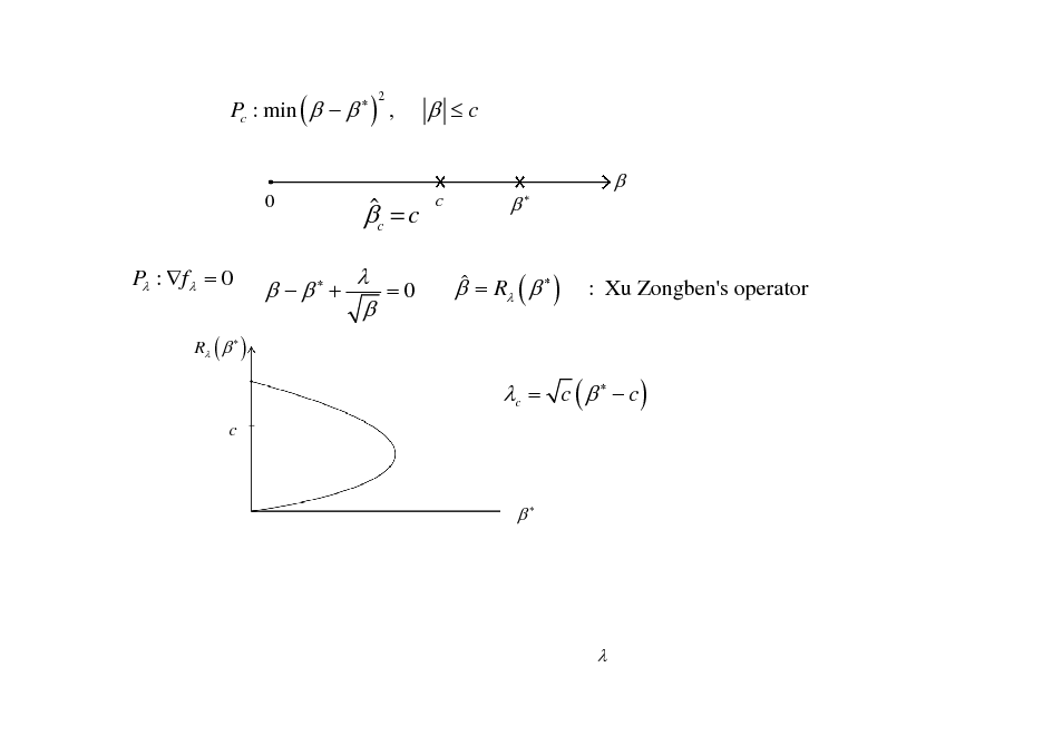
Pc : min ( ) ,
2
c
0
c = c
=0
c
P : f = 0
R ( )
+
= R ( )
: Xu Zongben's operator
c = c ( c )
c
82

ICCN-Huangshan
Sparse Signal Analysis
Shun-ichi Ammari
RIKEN Brain Science Institute Collaborator: Masahiro Yukawa, Niigata University)
83
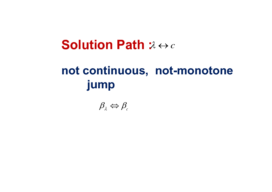
Solution Path : c
not continuous, not-monotone jump
c
84
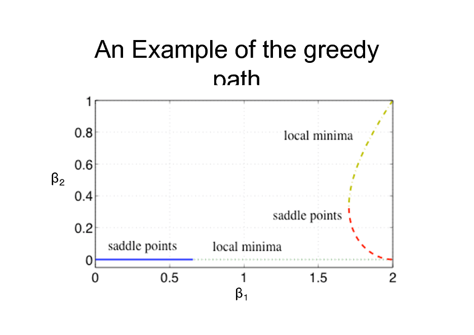
An Example of the greedy path
85
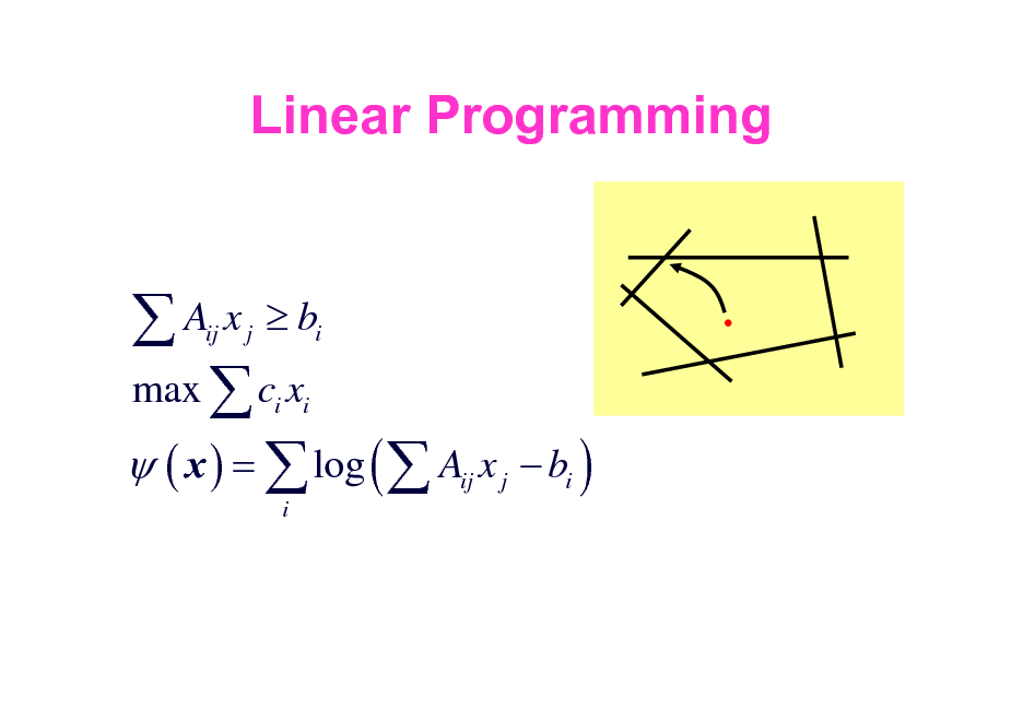
Linear Programming
A x b max c x ( x ) = log ( A x
ij j i i i ij i
j
bi )
inner method
86
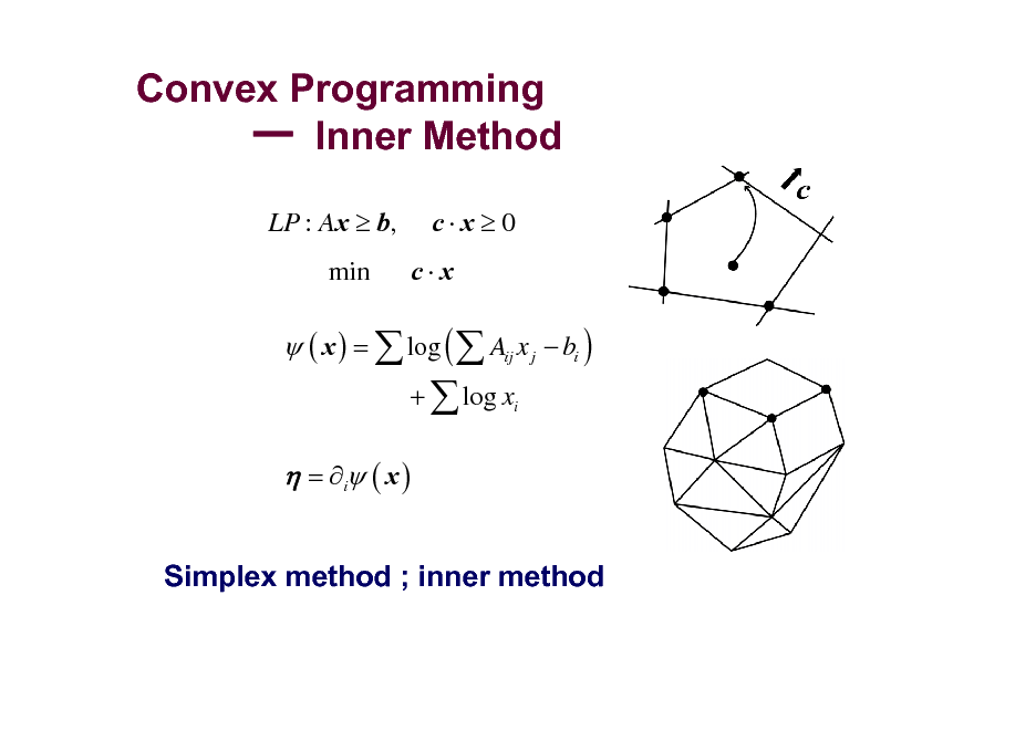
Convex Programming Inner Method
LP : Ax b,
min
c x 0
c x
( x ) = log ( Aij x j bi )
+ log xi
= i ( x )
Simplex method ; inner method
87
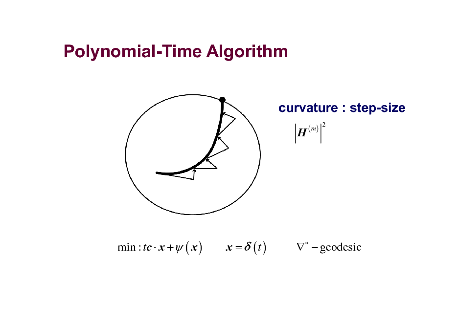
Polynomial-Time Algorithm
curvature : step-size
H
( m)
2
min : tc x + ( x )
x = (t )
geodesic
88
Neural Networks
Multilayer Perceptron Higher-order correlations
Synchronous firing
89
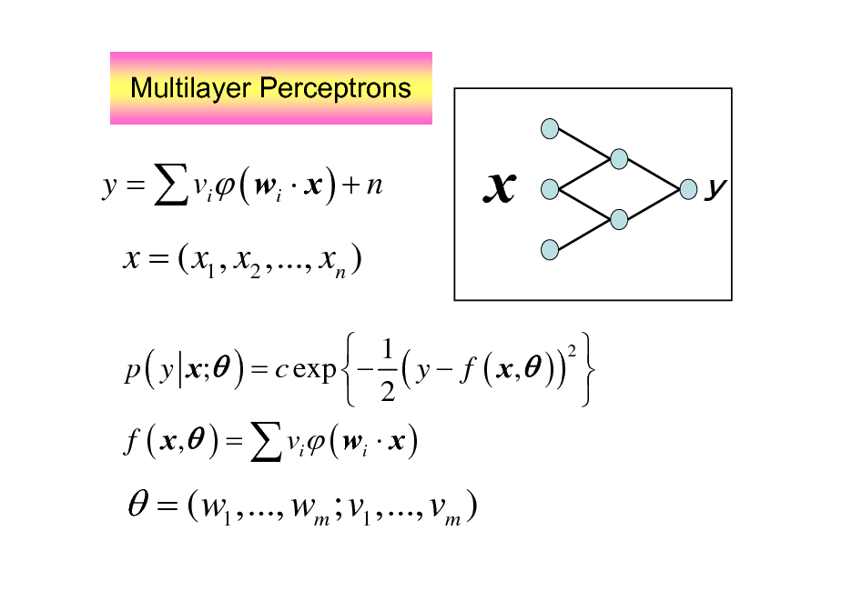
Multilayer Perceptrons
y = vi ( wi x ) + n
x
x = ( x1 , x2 ,..., xn )
2 1 p ( y x; ) = c exp ( y f ( x , ) ) 2 f ( x , ) = vi ( wi x )
= ( w1 ,..., wm ; v1 ,..., vm )
90
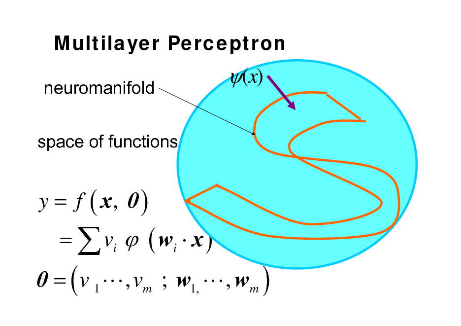
Multilayer Perceptron
neuromanifold space of functions
(x)
y = f ( x, ) = ( v 1 L , vm ; w1, L , wm ) = vi ( wi x )
91
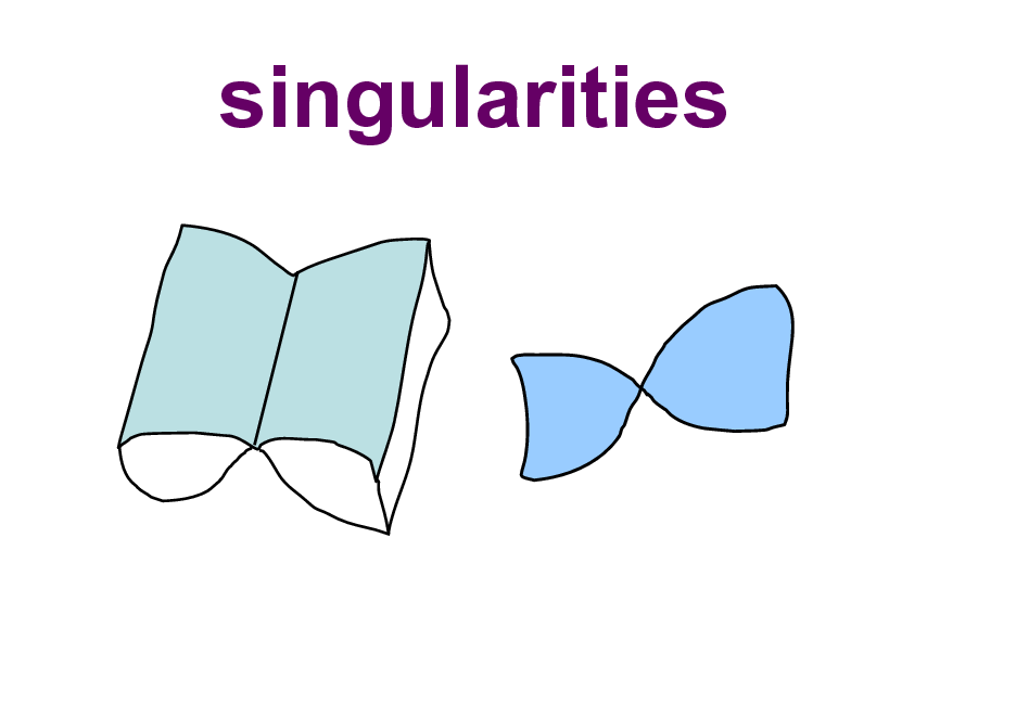
singularities
92
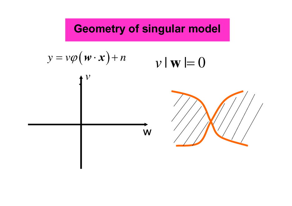
Geometry of singular model
y = v ( w x ) + n
v | w |= 0
v
93
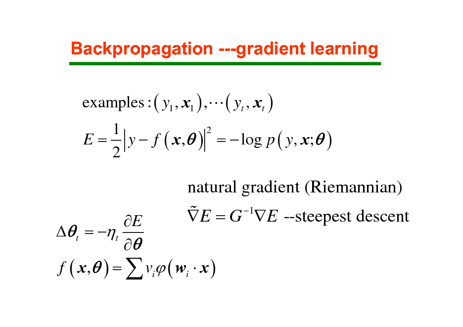
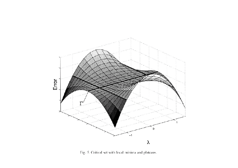
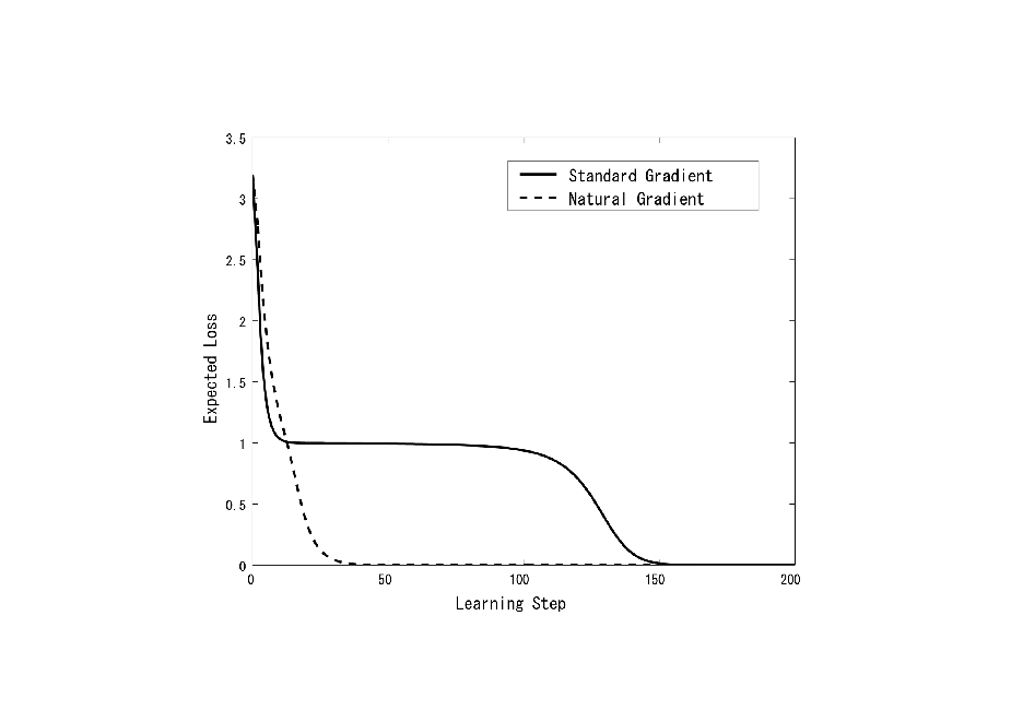
Backpropagation ---gradient learning
examples : ( y1 , x1 ) ,L ( yt , xt )
2 1 E = y f ( x , ) = log p ( y, x; ) 2
E t = t f ( x , ) = vi ( wi x )
natural gradient (Riemannian) % E = G 1E --steepest descent
94
95
96
![Slide: conformaltransformation
q Fisherinformation
q F gij ( p ) = gij ( p ) hq ( p )
(q)
q divergence 1 q 1q (1 p(x) r(x) dx) Dq[ p(x): r(x)] = (1 q)hq ( p)](https://yosinski.com/mlss12/media/slides/MLSS-2012-Amari-Information-Geometry_097.png)
conformaltransformation
q Fisherinformation
q F gij ( p ) = gij ( p ) hq ( p )
(q)
q divergence 1 q 1q (1 p(x) r(x) dx) Dq[ p(x): r(x)] = (1 q)hq ( p)
97
Total Bregman Divergence and its Applications to Shape Retrieval
Baba C. Vemuri, Meizhu Liu, Shun-ichi Amari, Frank Nielsen
IEEE Conference on Computer Vision and Pattern Recognition (CVPR), 2010
98
![Slide: Total Bregman Divergence
TD [ x : y ] = D [ x : y] 1 + f
2
rotational invariance conformal geometry](https://yosinski.com/mlss12/media/slides/MLSS-2012-Amari-Information-Geometry_099.png)
Total Bregman Divergence
TD [ x : y ] = D [ x : y] 1 + f
2
rotational invariance conformal geometry
99
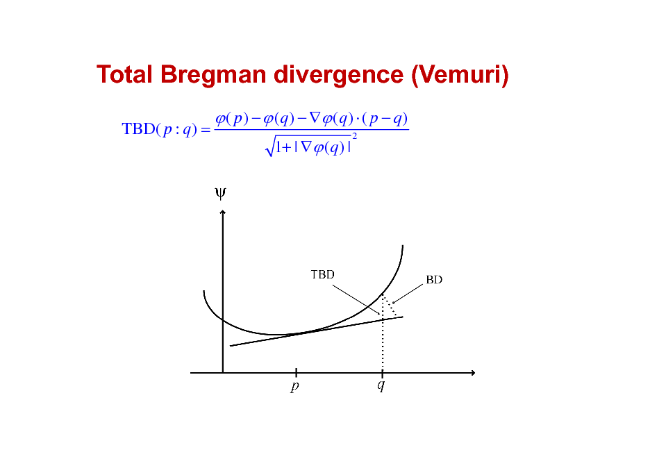
Total Bregman divergence (Vemuri)
TBD( p : q) =
( p ) ( q ) ( q ) ( p q )
1+ | (q ) |
2
100
![Slide: Clustering : t-center
y
E = { x1 ,L , xm }
T-center of E x = arg min TD [ x , xi ]
i
E
x](https://yosinski.com/mlss12/media/slides/MLSS-2012-Amari-Information-Geometry_101.png)
Clustering : t-center
y
E = { x1 ,L , xm }
T-center of E x = arg min TD [ x , xi ]
i
E
x
101
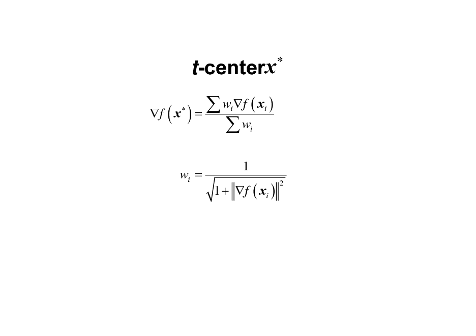
t-centerx
w f ( x ) f ( x ) = w
i i i
wi =
1 1 + f ( xi )
2
102
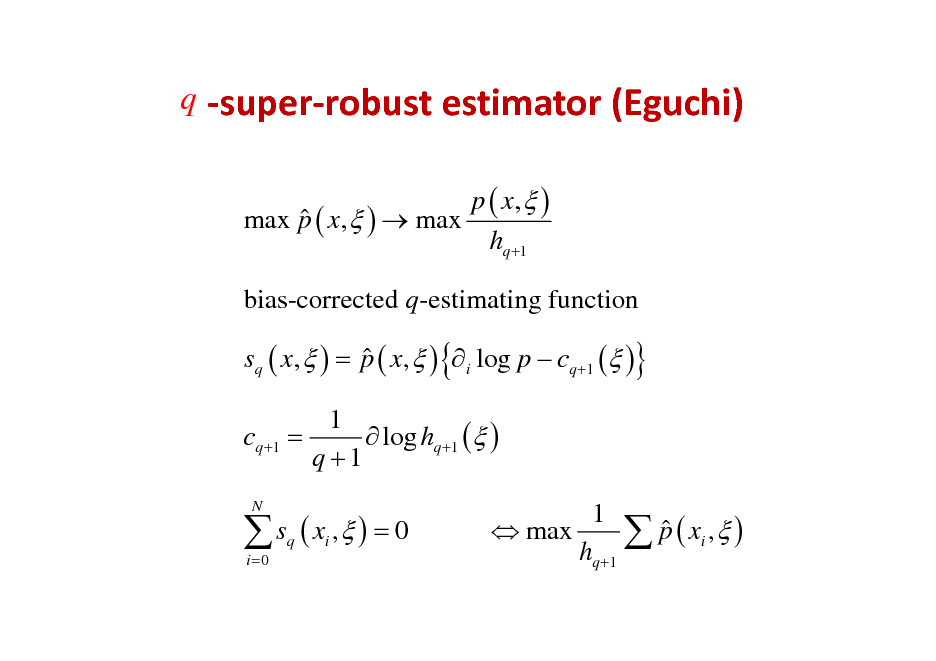
q superrobustestimator(Eguchi)
p ( x, ) max p ( x, ) max hq +1 bias-corrected q-estimating function sq ( x, ) = p ( x, ) { i log p cq +1 ( )} 1 cq +1 = log hq +1 ( ) q +1
s ( x , ) = 0
i =0 q i
N
1 max p ( xi , ) hq +1
103
![Slide: Conformalchangeofdivergence
% D ( p : q ) = ( p ) D [ p : q]
% gij = ( p ) gij
% Tijk = (Tijk + sk gij + s j gik + si g jk ) si = i log](https://yosinski.com/mlss12/media/slides/MLSS-2012-Amari-Information-Geometry_104.png)
Conformalchangeofdivergence
% D ( p : q ) = ( p ) D [ p : q]
% gij = ( p ) gij
% Tijk = (Tijk + sk gij + s j gik + si g jk ) si = i log
104
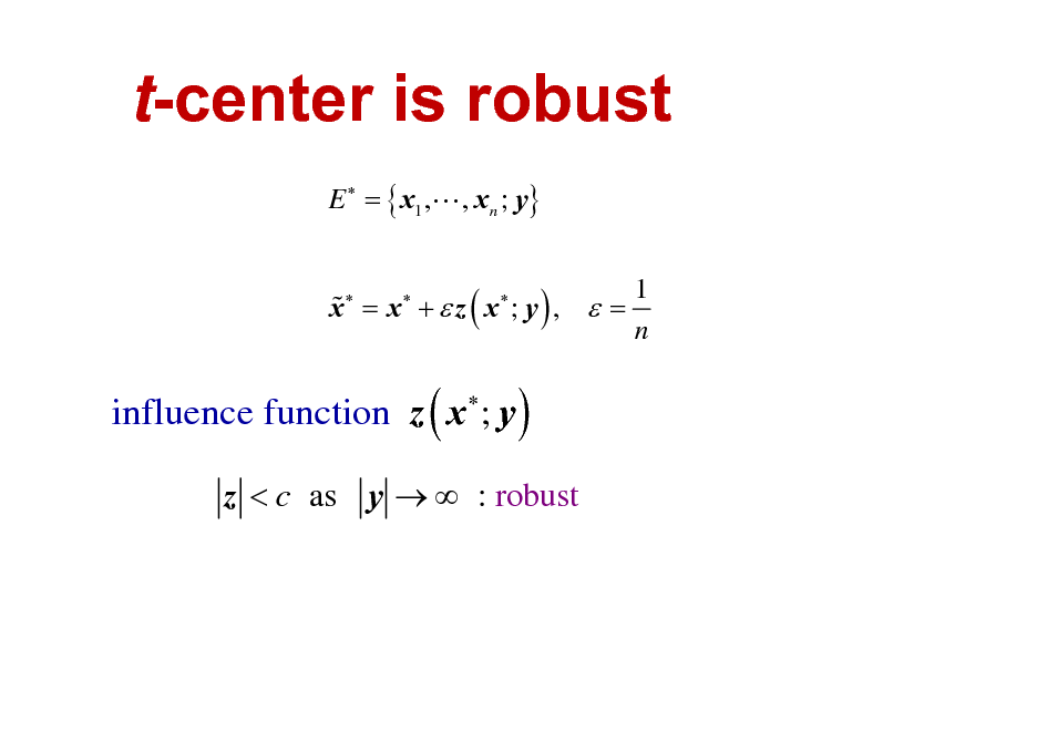
t-center is robust
E = { x1 ,L , xn ; y} % x = x + z ( x ; y ) , = 1 n
influence function z ( x ; y )
z < c as y : robust
105
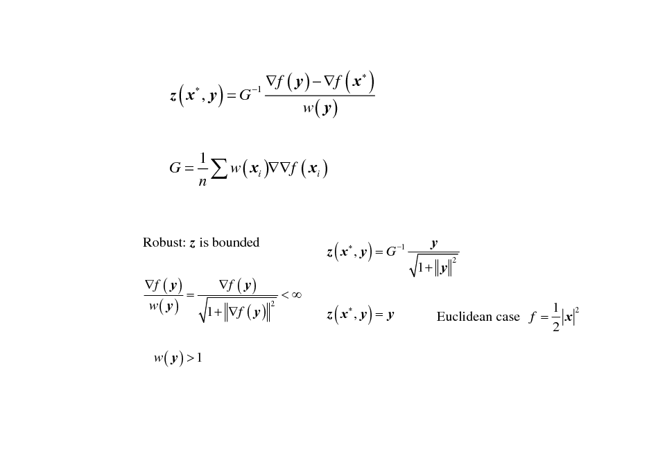
z ( x , y ) = G
f ( y ) f ( x ) 1 w( y)
1 G = w ( xi )f ( xi ) n
Robust: z is bounded f ( y ) f ( y ) = w( y) 1 + f ( y ) w( y) > 1
z ( x , y ) = G 1 <
y 1+ y
2
2
z ( x , y ) = y
Euclidean case f =
1 2 x 2
106
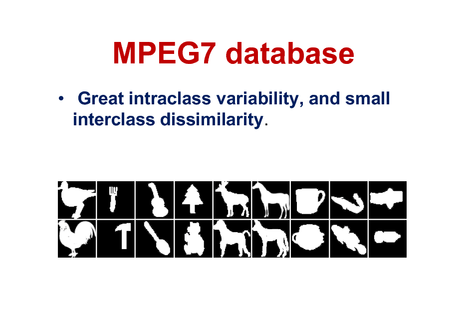
MPEG7 database
Great intraclass variability, and small interclass dissimilarity.
107
![Slide: Other TBD applications
Diffusion tensor imaging (DTI) analysis
[Vemuri]
Interpolation Segmentation
Baba C. Vemuri, Meizhu Liu, Shun-ichi Amari and Frank Nielsen, Total Bregman Divergence and its Applications to DTI Analysis, IEEE TMI, to appear](https://yosinski.com/mlss12/media/slides/MLSS-2012-Amari-Information-Geometry_108.png)
Other TBD applications
Diffusion tensor imaging (DTI) analysis
[Vemuri]
Interpolation Segmentation
Baba C. Vemuri, Meizhu Liu, Shun-ichi Amari and Frank Nielsen, Total Bregman Divergence and its Applications to DTI Analysis, IEEE TMI, to appear
108
TBD application-shape retrieval
Using MPEG7 database; 70 classes, with 20 shapes each class (Meizhu Liu)
109
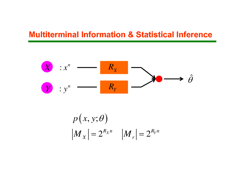
Multiterminal Information & Statistical Inference
X
Y
:x
n
RX RY
: yn
p ( x, y; ) M X = 2 RX n M r = 2 RY n
110
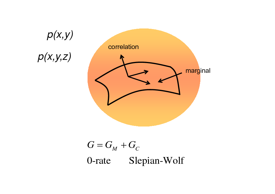
p(x,y)
correlation
p(x,y,z)
marginal
G = GM + GC 0-rate Slepian-Wolf
111
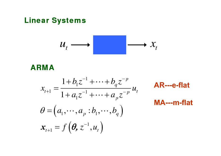
Linear Systems
ut
ARMA
xt
1 p
xt +1 =
1 + b1 z + L + bq z
= ( a1 ,L , a p : b1 ,L , bq )
xt +1 = f (, z 1 , ut )
1 + a1 z 1 + L + a p z p
ut
AR---e-flat MA---m-flat
112
Machine Learning
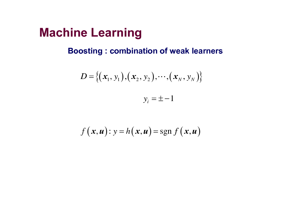
Boosting : combination of weak learners
D = {( x1 , y1 ) , ( x2 , y2 ) ,L , ( x N , yN )}
yi = 1
f ( x , u ) : y = h ( x , u ) = sgn f ( x , u )
113
Weak Learners
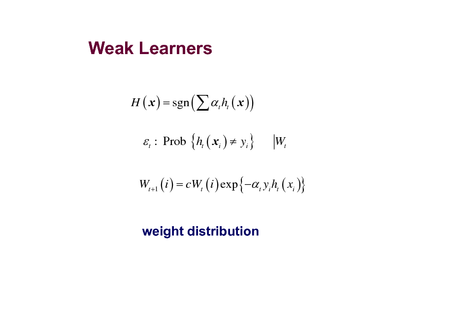
H ( x ) = sgn ( t ht ( x ) )
t : Prob {ht ( xi ) yi }
Wt
Wt +1 ( i ) = cWt ( i ) exp { t yi ht ( xi )}
weight distribution
114
Boosting generalization
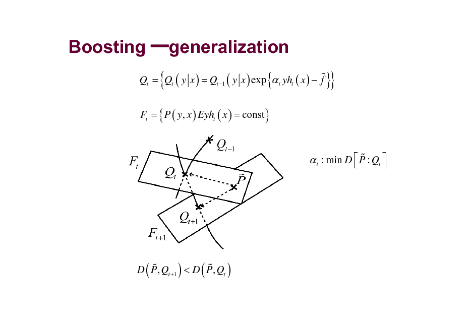
% Qt = Qt ( y x ) = Qt 1 ( y x ) exp t yht ( x ) f
Ft = { P ( y, x ) Eyht ( x ) = const}
{
{
}}
% t : min D P : Qt
% % D P, Qt +1 < D P, Qt
(
)
(
)
115
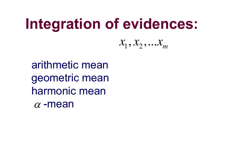
Integration of evidences:
x1 , x2 ,...xm
arithmetic mean geometric mean harmonic mean -mean
116
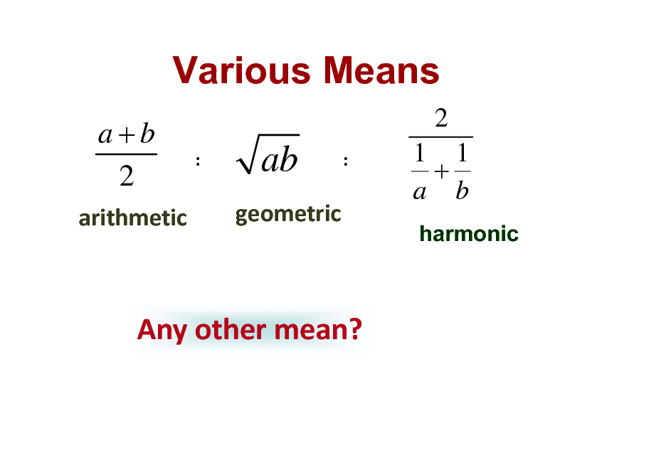
Various Means
a+b 2
arithmetic
2
:
ab
geometric
:
1 1 + a b
harmonic
Anyothermean?
117
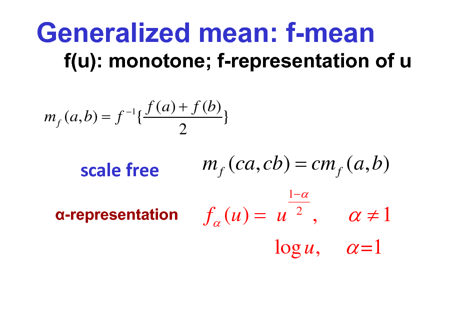
Generalized mean: f-mean
f(u): monotone; f-representation of u
f (a ) + f (b) m f ( a, b) = f { } 2
1
scalefree
-representation
m f (ca, cb) = cm f (a, b) f (u ) = u
1 2
,
log u ,
1 =1
118
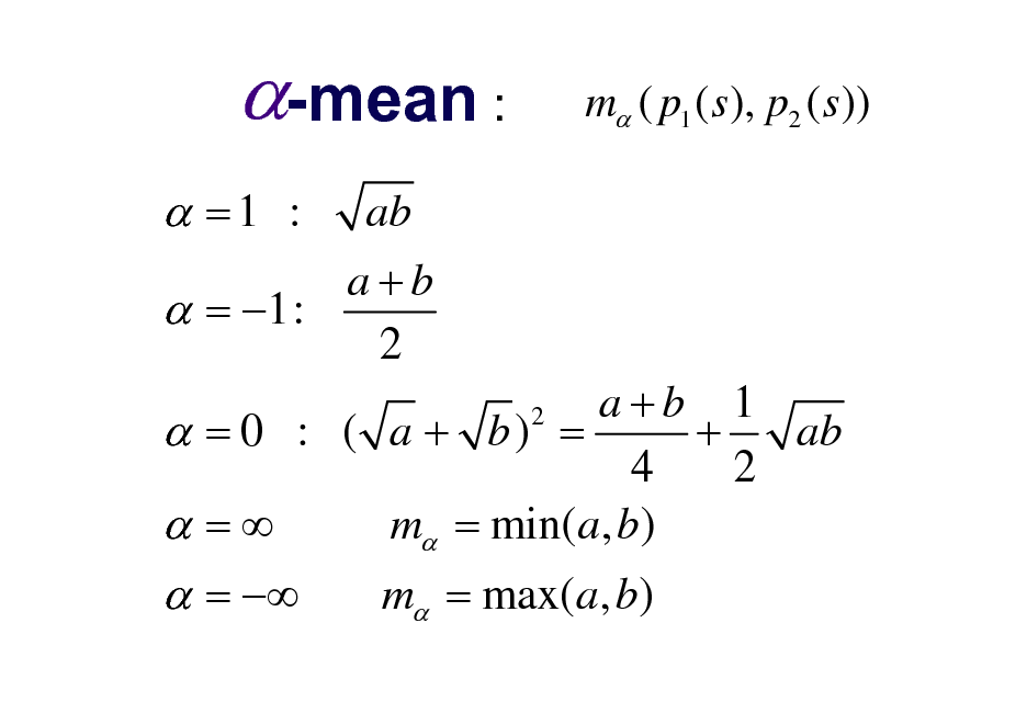
-mean :
=1 :
ab a+b = 1: 2
m ( p1 ( s ), p2 ( s ))
a+b 1 ab = 0 : ( a + b) = + 4 2 m = min(a, b) =
2
=
m = max(a, b)
119
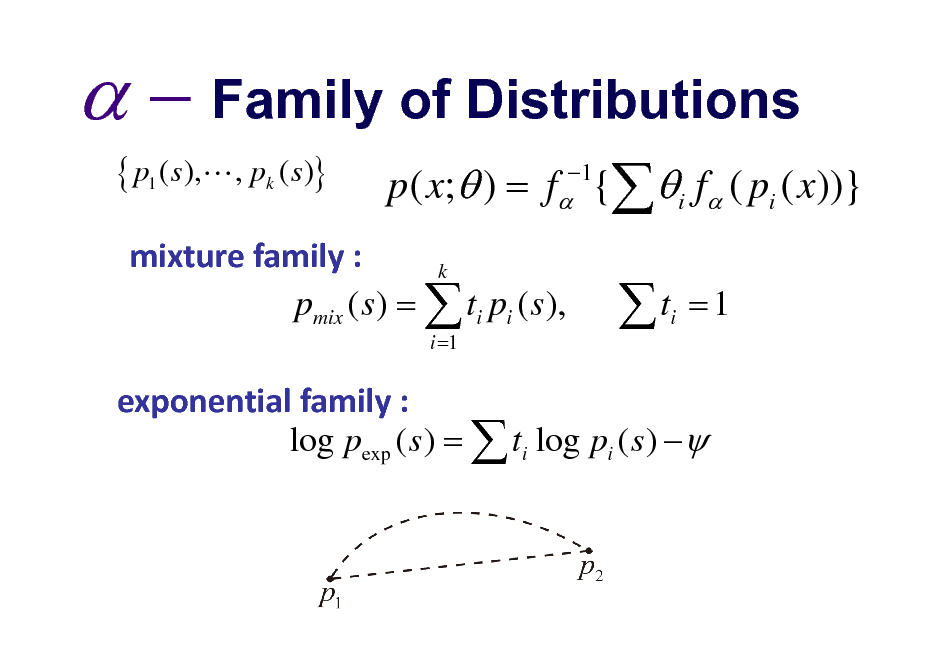
Family of Distributions
{ p1 ( s),L , pk ( s)}
p ( x; ) = f { i f ( pi ( x))}
1
mixturefamily: k pmix ( s ) = ti pi ( s ),
i =1
t
i
=1
exponentialfamily: log pexp ( s ) = ti log pi ( s )
120
Site based on the django-slidedeck framework by Jason Yosinski.
Find a bug? Email Jason or submit a pull request on Github.