
Learning with Submodular Functions
Francis Bach Sierra project-team, INRIA - Ecole Normale Suprieure e
Machine Learning Summer School, Kyoto September 2012
Submodular functions are relevant to machine learning for mainly two reasons: (1) some problems may be expressed directly as the optimization of submodular functions and (2) the Lovasz extension of submodular functions provides a useful set of regularization functions for supervised and unsupervised learning. In this course, I will present the theory of submodular functions from a convex analysis perspective, presenting tight links between certain polyhedra, combinatorial optimization and convex optimization problems. In particular, I will show how submodular function minimization is equivalent to solving a wide variety of convex optimization problems. This allows the derivation of new efficient algorithms for approximate submodular function minimization with theoretical guarantees and good practical performance. By listing examples of submodular functions, I will also review various applications to machine learning, such as clustering or subset selection, as well as a family of structured sparsity-inducing norms that can be derived and used from submodular functions.
Scroll with j/k | | | Size

Learning with Submodular Functions
Francis Bach Sierra project-team, INRIA - Ecole Normale Suprieure e
Machine Learning Summer School, Kyoto September 2012
1
Submodular functions- References and Links
References based on from combinatorial optimization Submodular Functions and Optimization (Fujishige, 2005) Discrete convex analysis (Murota, 2003) Tutorial paper based on convex optimization (Bach, 2011) www.di.ens.fr/~fbach/submodular_fot.pdf Slides for this class www.di.ens.fr/~fbach/submodular_fbach_mlss2012.pdf Other tutorial slides and code at submodularity.org/ Lecture slides at ssli.ee.washington.edu/~ bilmes/ee595a_ spring_2011/
2

Submodularity (almost) everywhere Clustering
Semi-supervised clustering
Submodular function minimization
3
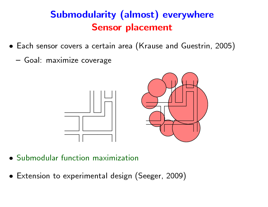
Submodularity (almost) everywhere Sensor placement
Each sensor covers a certain area (Krause and Guestrin, 2005) Goal: maximize coverage
Submodular function maximization Extension to experimental design (Seeger, 2009)
4

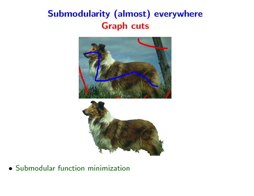
Submodularity (almost) everywhere Graph cuts
Submodular function minimization
5
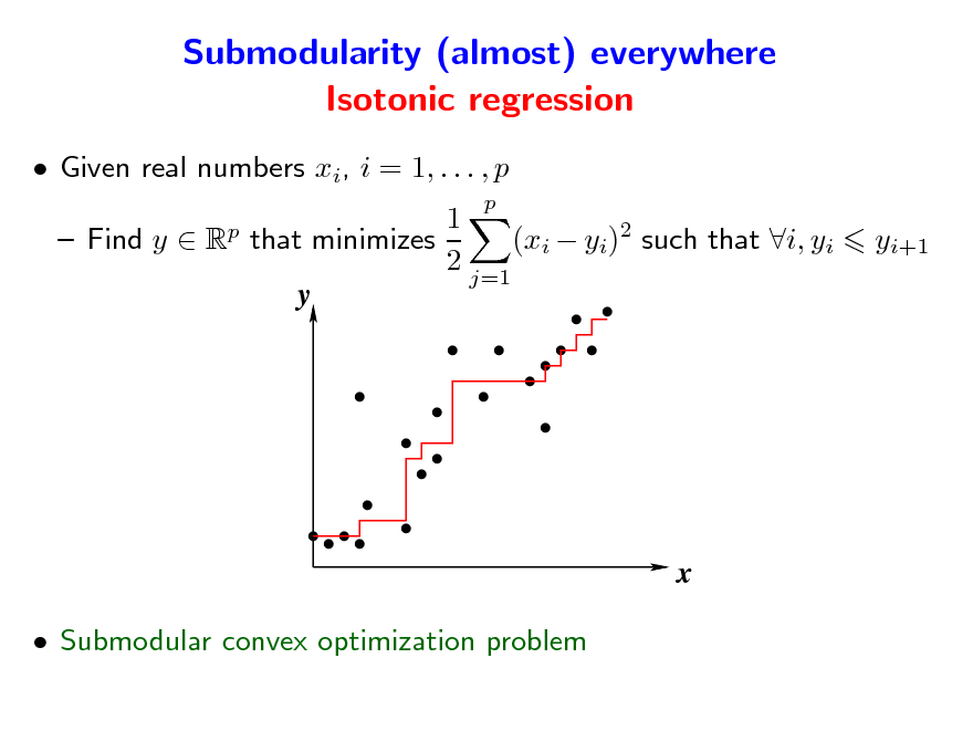
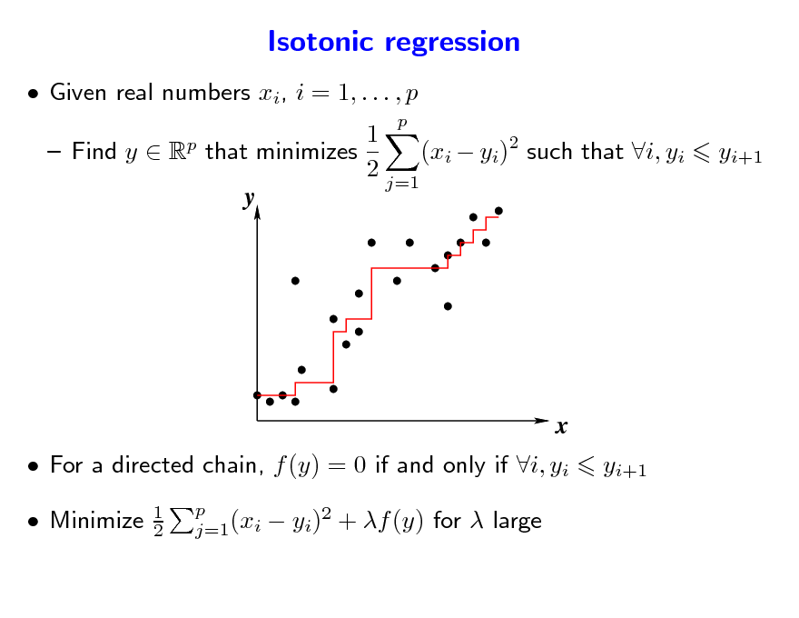
Submodularity (almost) everywhere Isotonic regression
Given real numbers xi, i = 1, . . . , p
p p
1 Find y R that minimizes (xi yi)2 such that i, yi 2 j=1 y
yi+1
x
Submodular convex optimization problem
6
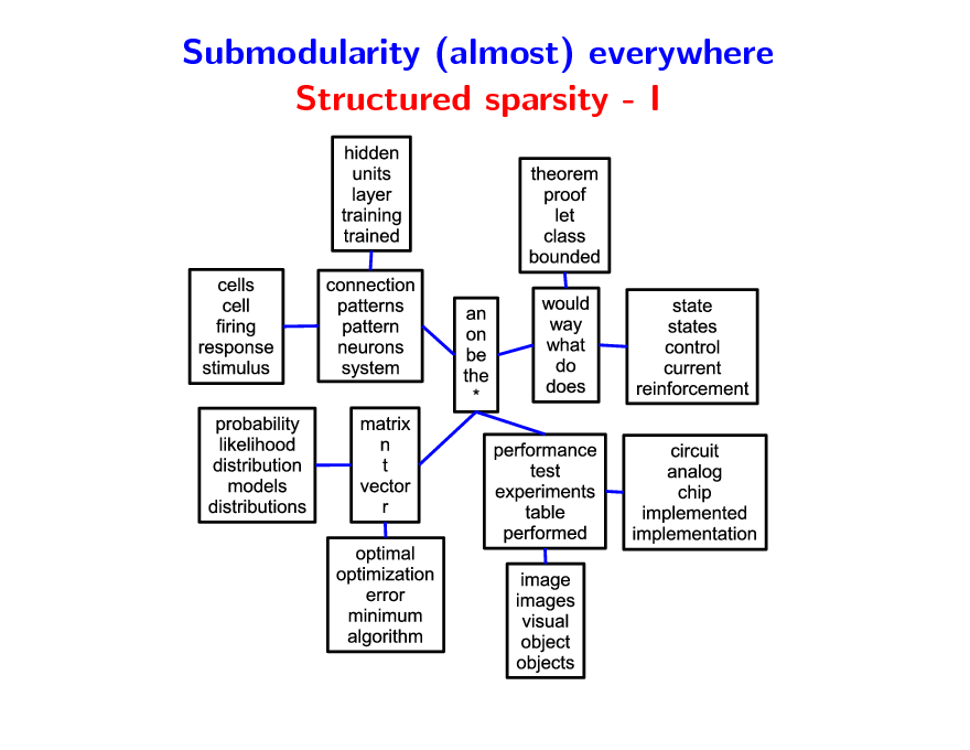
Submodularity (almost) everywhere Structured sparsity - I
7
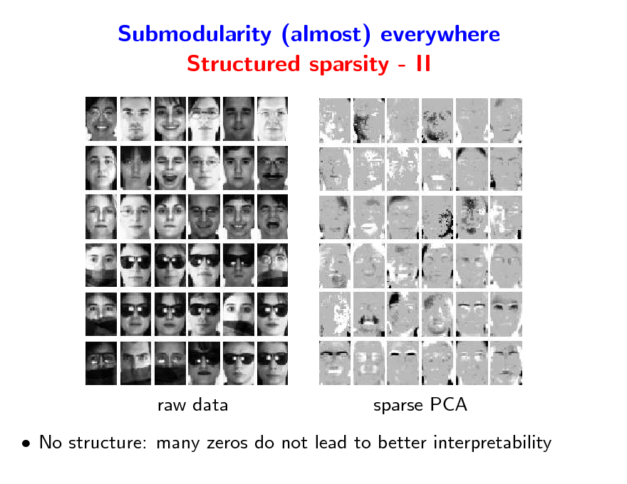
Submodularity (almost) everywhere Structured sparsity - II
raw data
sparse PCA
No structure: many zeros do not lead to better interpretability
8
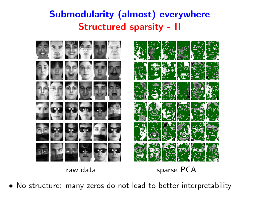
Submodularity (almost) everywhere Structured sparsity - II
raw data
sparse PCA
No structure: many zeros do not lead to better interpretability
9
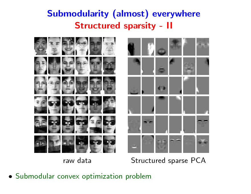
Submodularity (almost) everywhere Structured sparsity - II
raw data
Structured sparse PCA
Submodular convex optimization problem
10
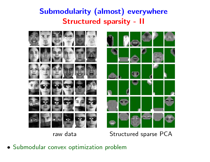
Submodularity (almost) everywhere Structured sparsity - II
raw data
Structured sparse PCA
Submodular convex optimization problem
11
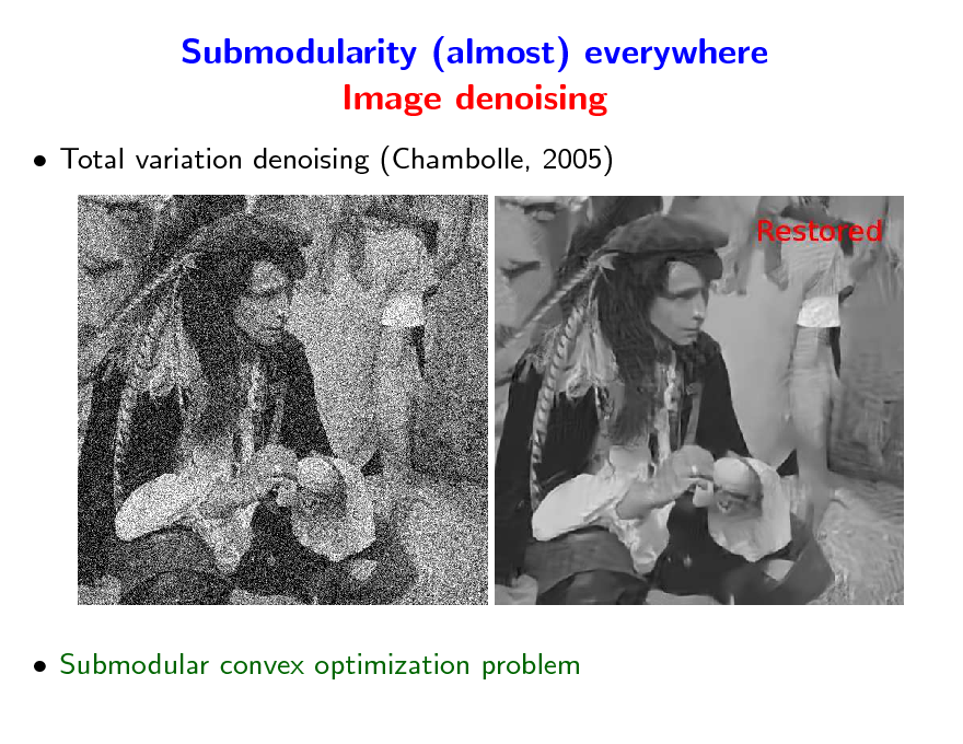
Submodularity (almost) everywhere Image denoising
Total variation denoising (Chambolle, 2005)
Submodular convex optimization problem
12
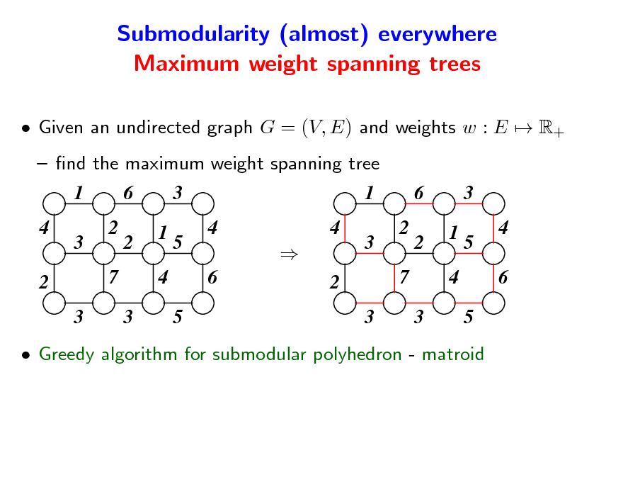
Submodularity (almost) everywhere Maximum weight spanning trees
Given an undirected graph G = (V, E) and weights w : E R+ nd the maximum weight spanning tree
1 4 2 3 3 2 7
6 2 1 4 3
3 5 4 6 5
1 4 2 3 3 2 7
6 2 1 4 3
3 5 4 6 5
Greedy algorithm for submodular polyhedron - matroid
13
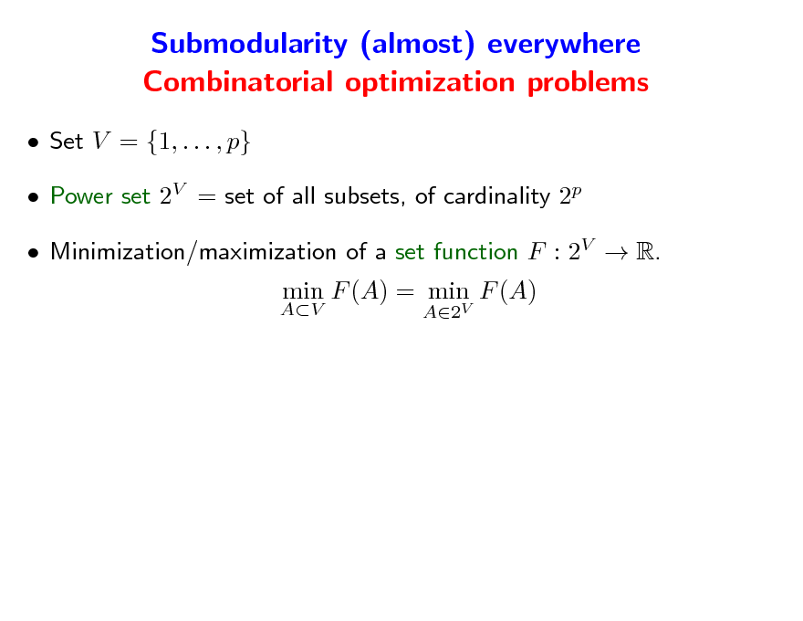
Submodularity (almost) everywhere Combinatorial optimization problems
Set V = {1, . . . , p} Power set 2V = set of all subsets, of cardinality 2p Minimization/maximization of a set function F : 2V R.
AV
min F (A) = min F (A)
A2V
14
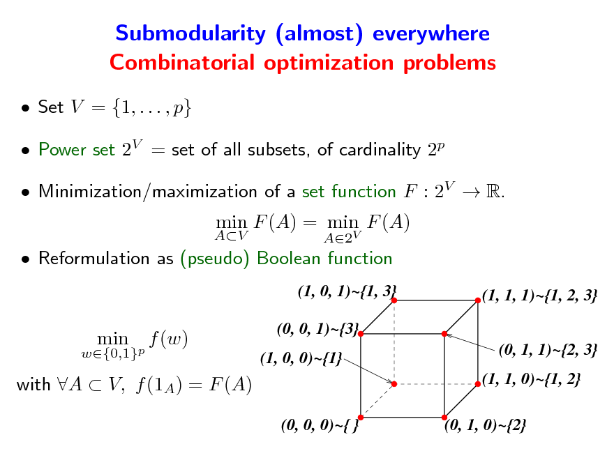
Submodularity (almost) everywhere Combinatorial optimization problems
Set V = {1, . . . , p} Power set 2V = set of all subsets, of cardinality 2p Minimization/maximization of a set function F : 2V R.
AV
min F (A) = min F (A)
A2V
Reformulation as (pseudo) Boolean function
(1, 0, 1)~{1, 3} (1, 1, 1)~{1, 2, 3} (0, 1, 1)~{2, 3} (1, 1, 0)~{1, 2} (0, 0, 0)~{ } (0, 1, 0)~{2}
w{0,1}p
min
f (w)
(0, 0, 1)~{3} (1, 0, 0)~{1}
with A V, f (1A) = F (A)
15
Submodularity (almost) everywhere Convex optimization with combinatorial structure
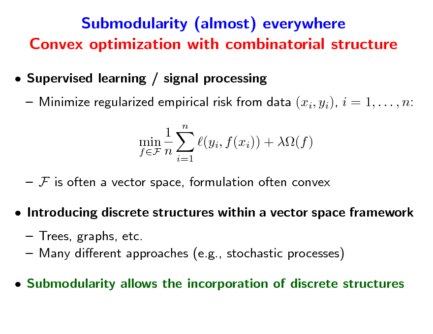
Supervised learning / signal processing Minimize regularized empirical risk from data (xi, yi), i = 1, . . . , n: 1 min (yi, f (xi)) + (f ) f F n i=1 F is often a vector space, formulation often convex Introducing discrete structures within a vector space framework Trees, graphs, etc. Many dierent approaches (e.g., stochastic processes) Submodularity allows the incorporation of discrete structures
n
16

Outline
1. Submodular functions Denitions Examples of submodular functions Links with convexity through Lovsz extension a 2. Submodular optimization Minimization Links with convex optimization Maximization 3. Structured sparsity-inducing norms Norms with overlapping groups Relaxation of the penalization of supports by submodular functions
17
Submodular functions Denitions
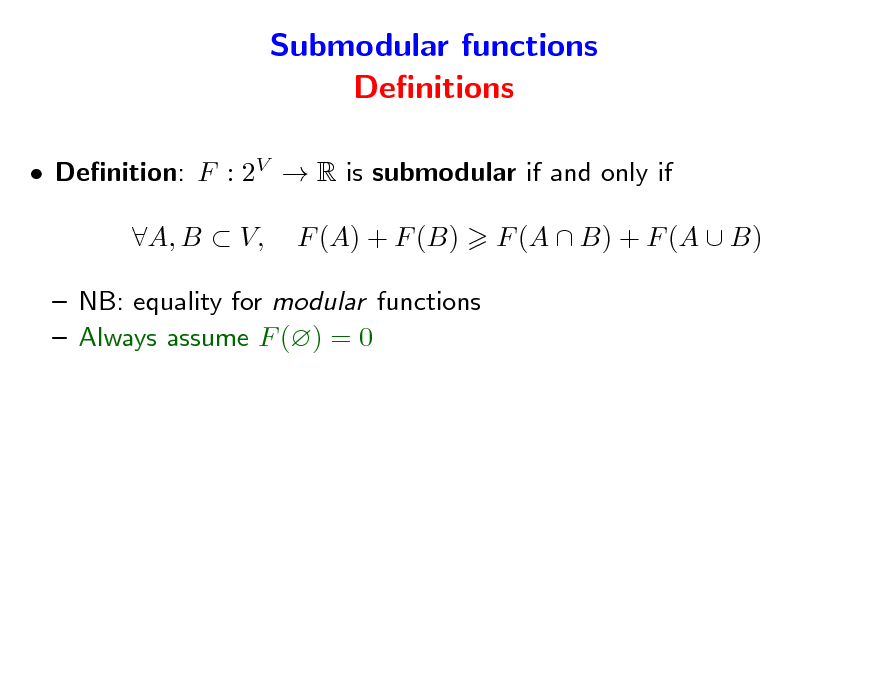
Denition: F : 2V R is submodular if and only if A, B V, F (A) + F (B) F (A B) + F (A B)
NB: equality for modular functions Always assume F () = 0
18
Submodular functions Denitions
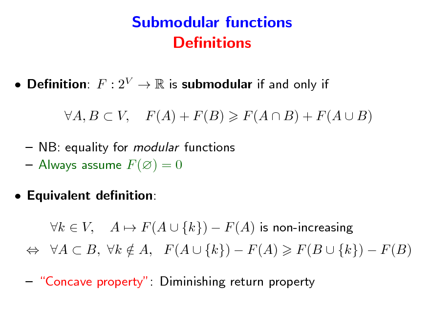
Denition: F : 2V R is submodular if and only if A, B V, F (A) + F (B) F (A B) + F (A B)
NB: equality for modular functions Always assume F () = 0 Equivalent denition: A B, k A, F (A {k}) F (A) / k V, A F (A {k}) F (A) is non-increasing F (B {k}) F (B)
Concave property: Diminishing return property
19
Submodular functions Denitions
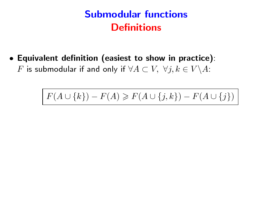
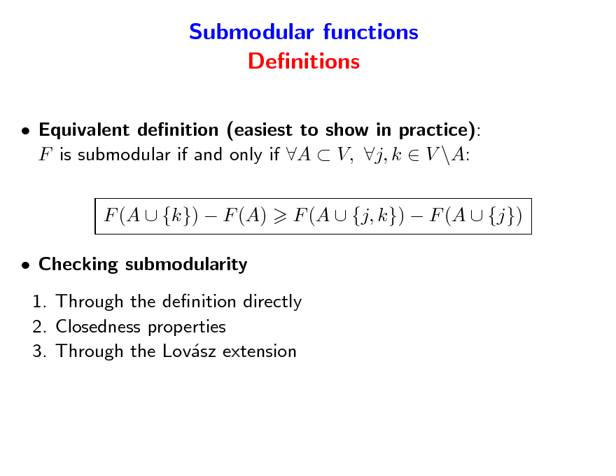
Equivalent denition (easiest to show in practice): F is submodular if and only if A V, j, k V \A: F (A {k}) F (A) F (A {j, k}) F (A {j})
20
Submodular functions Denitions
Equivalent denition (easiest to show in practice): F is submodular if and only if A V, j, k V \A: F (A {k}) F (A) Checking submodularity 1. Through the denition directly 2. Closedness properties 3. Through the Lovsz extension a F (A {j, k}) F (A {j})
21
Submodular functions Closedness properties
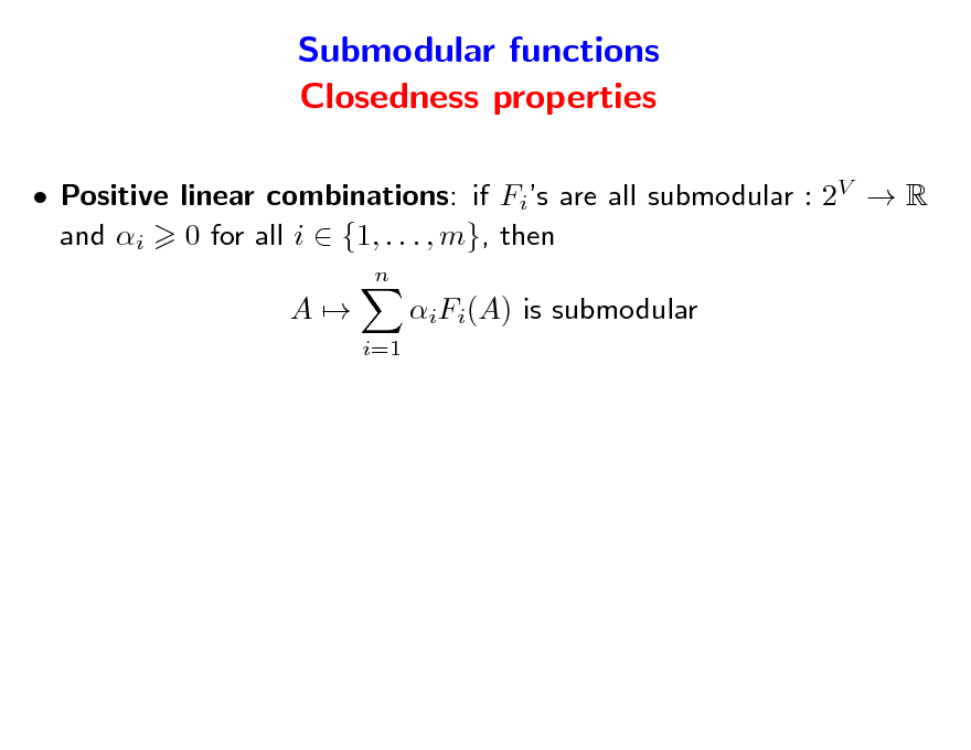
Positive linear combinations: if Fis are all submodular : 2V R and i 0 for all i {1, . . . , m}, then
n
A
iFi(A) is submodular
i=1
22
Submodular functions Closedness properties
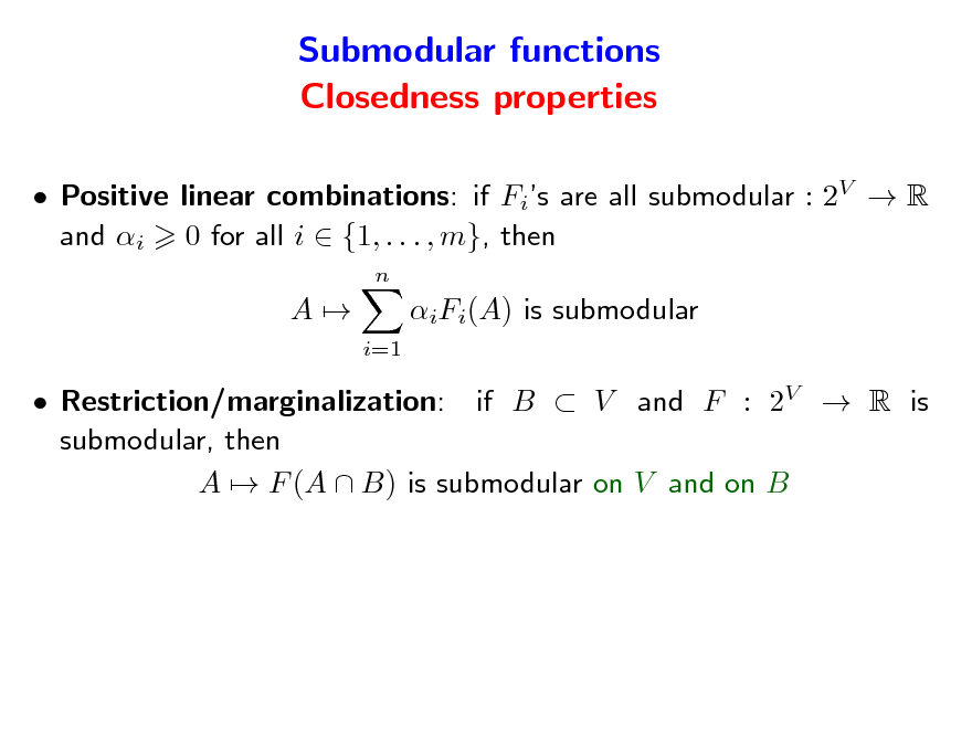
Positive linear combinations: if Fis are all submodular : 2V R and i 0 for all i {1, . . . , m}, then
n
A
iFi(A) is submodular
i=1
Restriction/marginalization: if B V and F : 2V R is submodular, then A F (A B) is submodular on V and on B
23
Submodular functions Closedness properties
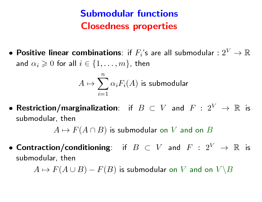
Positive linear combinations: if Fis are all submodular : 2V R and i 0 for all i {1, . . . , m}, then
n
A
iFi(A) is submodular
i=1
Restriction/marginalization: if B V and F : 2V R is submodular, then A F (A B) is submodular on V and on B Contraction/conditioning: if B V and F : 2V R is submodular, then A F (A B) F (B) is submodular on V and on V \B
24
Submodular functions Partial minimization
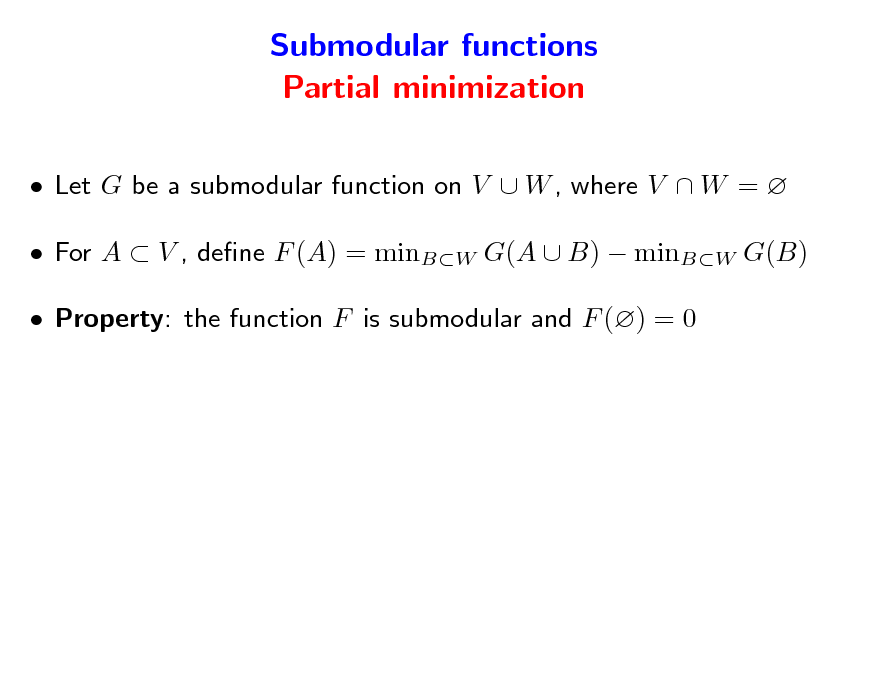
Let G be a submodular function on V W , where V W = For A V , dene F (A) = minBW G(A B) minBW G(B) Property: the function F is submodular and F () = 0
25
Submodular functions Partial minimization
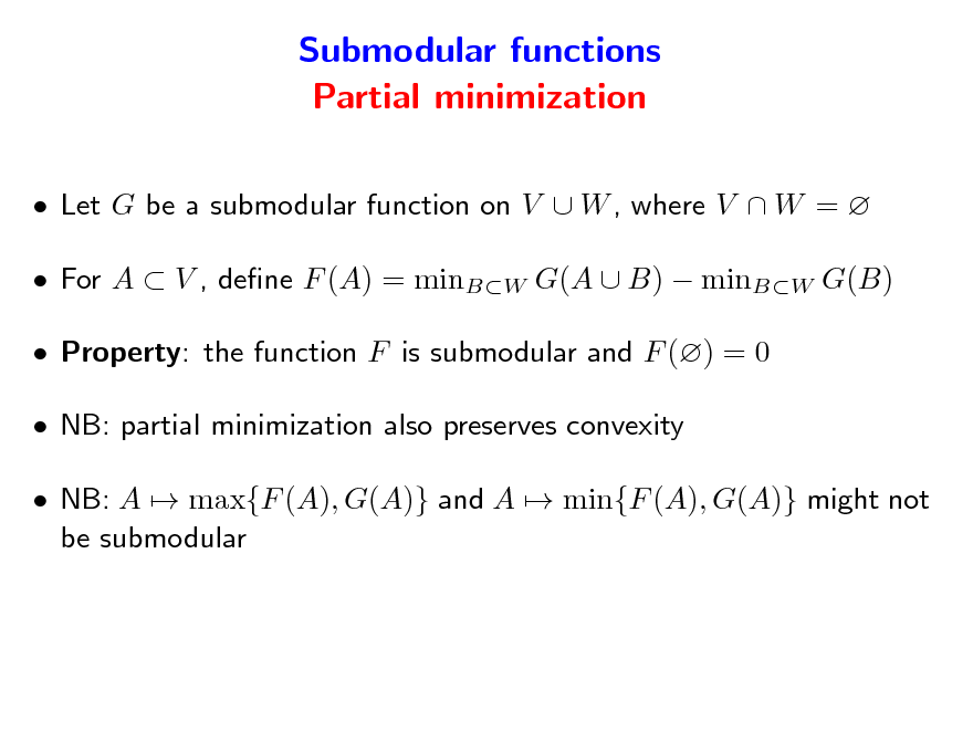
Let G be a submodular function on V W , where V W = For A V , dene F (A) = minBW G(A B) minBW G(B) Property: the function F is submodular and F () = 0 NB: partial minimization also preserves convexity NB: A max{F (A), G(A)} and A min{F (A), G(A)} might not be submodular
26
Examples of submodular functions Cardinality-based functions
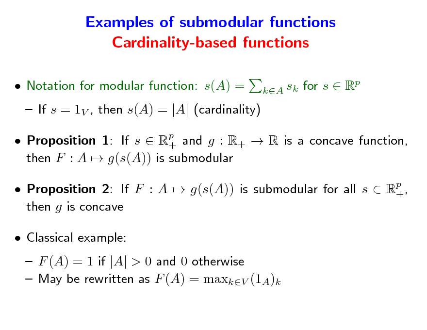
Notation for modular function: s(A) = If s = 1V , then s(A) = |A| (cardinality) Proposition 1: If s Rp and g : R+ R is a concave function, + then F : A g(s(A)) is submodular Proposition 2: If F : A g(s(A)) is submodular for all s Rp , + then g is concave Classical example: F (A) = 1 if |A| > 0 and 0 otherwise May be rewritten as F (A) = maxkV (1A)k sk for s Rp kA
27
Examples of submodular functions Covers
S4 S3 S5 S6 S7 S8
S2 S1
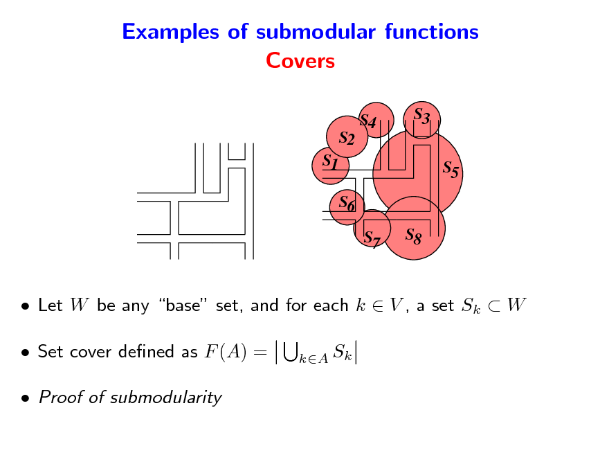
Let W be any base set, and for each k V , a set Sk W Set cover dened as F (A) = Proof of submodularity
kA Sk
28
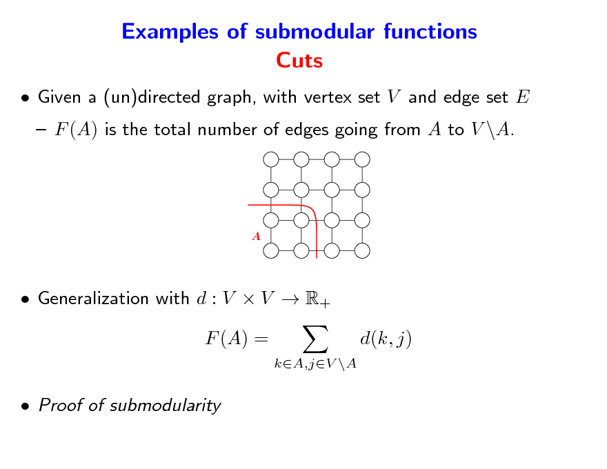
Examples of submodular functions Cuts
Given a (un)directed graph, with vertex set V and edge set E F (A) is the total number of edges going from A to V \A.
A
Generalization with d : V V R+ F (A) =
kA,jV \A
d(k, j)
Proof of submodularity
29
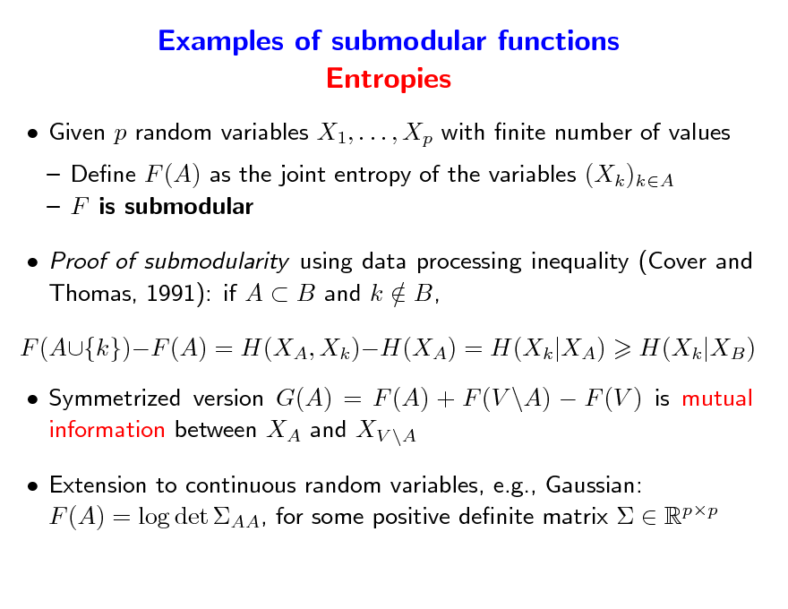
Examples of submodular functions Entropies
Given p random variables X1, . . . , Xp with nite number of values Dene F (A) as the joint entropy of the variables (Xk )kA F is submodular Proof of submodularity using data processing inequality (Cover and Thomas, 1991): if A B and k B, / F (A{k})F (A) = H(XA, Xk )H(XA) = H(Xk |XA) H(Xk |XB )
Symmetrized version G(A) = F (A) + F (V \A) F (V ) is mutual information between XA and XV \A Extension to continuous random variables, e.g., Gaussian: F (A) = log det AA, for some positive denite matrix Rpp
30
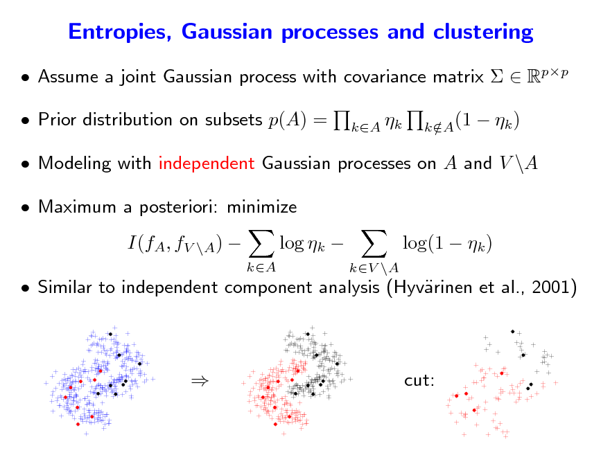
Entropies, Gaussian processes and clustering
Assume a joint Gaussian process with covariance matrix Rpp Prior distribution on subsets p(A) =
kA k kA(1 /
k )
Modeling with independent Gaussian processes on A and V \A Maximum a posteriori: minimize I(fA, fV \A)
kA
log k
Similar to independent component analysis (Hyvrinen et al., 2001) a
kV \A
log(1 k )
cut:
31
Examples of submodular functions Flows
Net-ows from multi-sink multi-source networks (Megiddo, 1974) See details in www.di.ens.fr/~ fbach/submodular_fot.pdf Ecient formulation for set covers
32
Examples of submodular functions Matroids
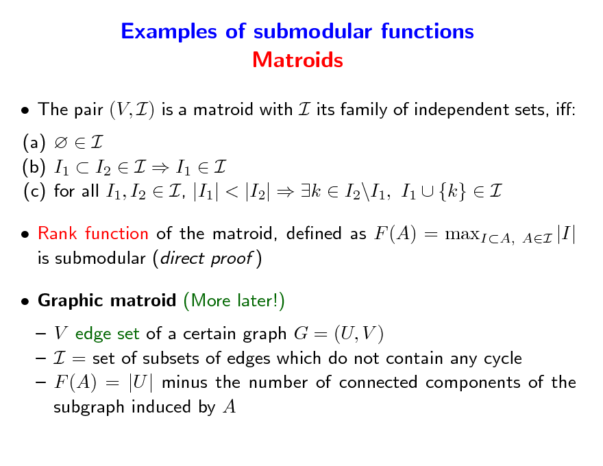
The pair (V, I) is a matroid with I its family of independent sets, i: (a) I (b) I1 I2 I I1 I (c) for all I1, I2 I, |I1| < |I2| k I2\I1, I1 {k} I Rank function of the matroid, dened as F (A) = maxIA, is submodular (direct proof ) Graphic matroid (More later!) V edge set of a certain graph G = (U, V ) I = set of subsets of edges which do not contain any cycle F (A) = |U | minus the number of connected components of the subgraph induced by A
AI
|I|
33
Outline
1. Submodular functions Denitions Examples of submodular functions Links with convexity through Lovsz extension a 2. Submodular optimization Minimization Links with convex optimization Maximization 3. Structured sparsity-inducing norms Norms with overlapping groups Relaxation of the penalization of supports by submodular functions
34
![Slide: Choquet integral - Lovsz extension a
Subsets may be identied with elements of {0, 1}p Given any set-function F and w such that wj1
p
wjp , dene:
f (w) =
k=1 p1
wjk [F ({j1, . . . , jk }) F ({j1, . . . , jk1})]
=
k=1
(wjk wjk+1 )F ({j1, . . . , jk }) + wjp F ({j1, . . . , jp})
(1, 0, 1)~{1, 3} (1, 1, 1)~{1, 2, 3} (0, 1, 1)~{2, 3} (1, 1, 0)~{1, 2}
(0, 0, 1)~{3} (1, 0, 0)~{1}
(0, 0, 0)~{ }
(0, 1, 0)~{2}](https://yosinski.com/mlss12/media/slides/MLSS-2012-Bach-Learning-with-Submodular-Functions_035.png)
Choquet integral - Lovsz extension a
Subsets may be identied with elements of {0, 1}p Given any set-function F and w such that wj1
p
wjp , dene:
f (w) =
k=1 p1
wjk [F ({j1, . . . , jk }) F ({j1, . . . , jk1})]
=
k=1
(wjk wjk+1 )F ({j1, . . . , jk }) + wjp F ({j1, . . . , jp})
(1, 0, 1)~{1, 3} (1, 1, 1)~{1, 2, 3} (0, 1, 1)~{2, 3} (1, 1, 0)~{1, 2}
(0, 0, 1)~{3} (1, 0, 0)~{1}
(0, 0, 0)~{ }
(0, 1, 0)~{2}
35
![Slide: Choquet integral - Lovsz extension a Properties
p
f (w) =
k=1 p1
wjk [F ({j1, . . . , jk }) F ({j1, . . . , jk1})]
=
k=1
(wjk wjk+1 )F ({j1, . . . , jk }) + wjp F ({j1, . . . , jp})
For any set-function F (even not submodular) f is piecewise-linear and positively homogeneous If w = 1A, f (w) = F (A) extension from {0, 1}p to Rp](https://yosinski.com/mlss12/media/slides/MLSS-2012-Bach-Learning-with-Submodular-Functions_036.png)
Choquet integral - Lovsz extension a Properties
p
f (w) =
k=1 p1
wjk [F ({j1, . . . , jk }) F ({j1, . . . , jk1})]
=
k=1
(wjk wjk+1 )F ({j1, . . . , jk }) + wjp F ({j1, . . . , jp})
For any set-function F (even not submodular) f is piecewise-linear and positively homogeneous If w = 1A, f (w) = F (A) extension from {0, 1}p to Rp
36
![Slide: Choquet integral - Lovsz extension a Example with p = 2
If w1 If w1 w2, f (w) = F ({1})w1 + [F ({1, 2}) F ({1})]w2 w2, f (w) = F ({2})w2 + [F ({1, 2}) F ({2})]w1
w2
w2 >w1 (0,1)/F({2}) f(w)=1 0
(1,1)/F({1,2}) w1 >w2 w1 (1,0)/F({1})
(level set {w R2, f (w) = 1} is displayed in blue) NB: Compact formulation f (w) = [F ({1})+F ({2})F ({1, 2})] min{w1, w2}+F ({1})w1+F ({2})w2](https://yosinski.com/mlss12/media/slides/MLSS-2012-Bach-Learning-with-Submodular-Functions_037.png)
Choquet integral - Lovsz extension a Example with p = 2
If w1 If w1 w2, f (w) = F ({1})w1 + [F ({1, 2}) F ({1})]w2 w2, f (w) = F ({2})w2 + [F ({1, 2}) F ({2})]w1
w2
w2 >w1 (0,1)/F({2}) f(w)=1 0
(1,1)/F({1,2}) w1 >w2 w1 (1,0)/F({1})
(level set {w R2, f (w) = 1} is displayed in blue) NB: Compact formulation f (w) = [F ({1})+F ({2})F ({1, 2})] min{w1, w2}+F ({1})w1+F ({2})w2
37
Submodular functions Links with convexity
Theorem (Lovsz, 1982): F is submodular if and only if f is convex a Proof requires additional notions: Submodular and base polyhedra
38
Submodular and base polyhedra - Denitions
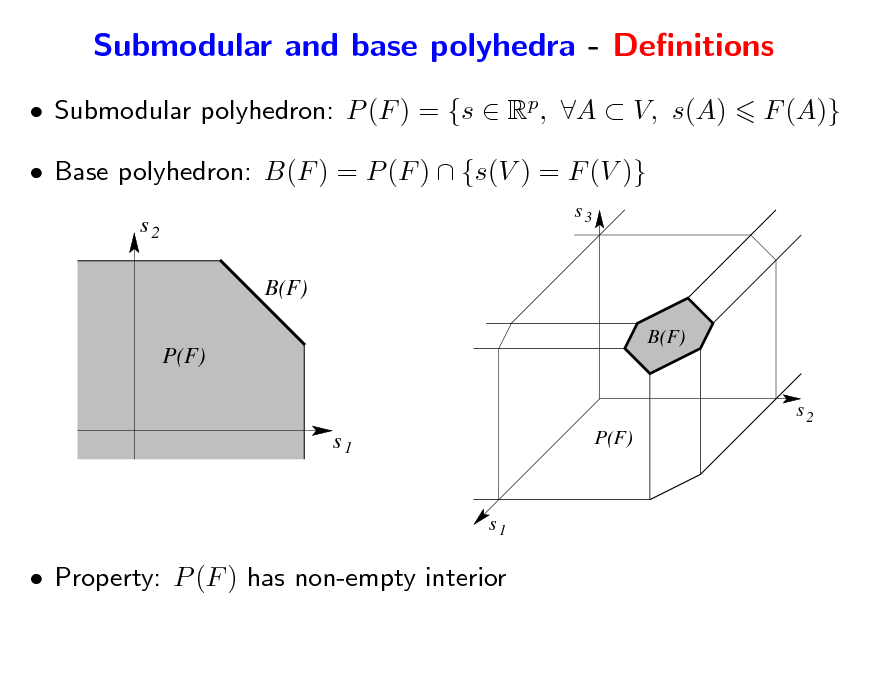
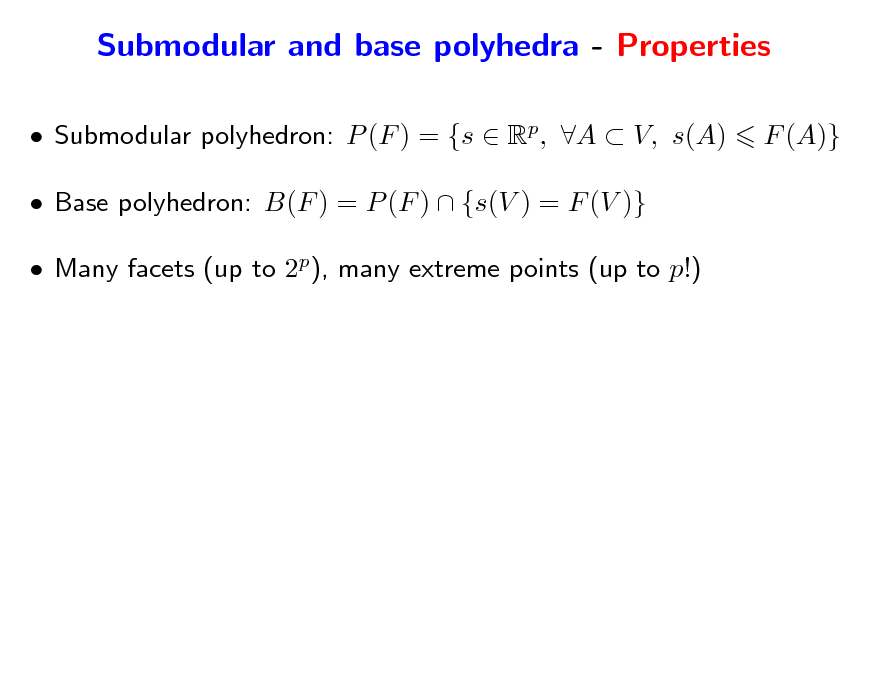
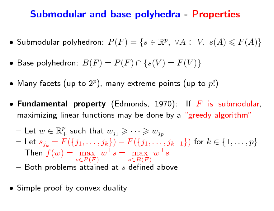
Submodular polyhedron: P (F ) = {s Rp, A V, s(A) Base polyhedron: B(F ) = P (F ) {s(V ) = F (V )}
s2 B(F) P(F)
B(F) s3
F (A)}
s2
s1
P(F)
s1
Property: P (F ) has non-empty interior
39
Submodular and base polyhedra - Properties
Submodular polyhedron: P (F ) = {s Rp, A V, s(A) Base polyhedron: B(F ) = P (F ) {s(V ) = F (V )} Many facets (up to 2p), many extreme points (up to p!) F (A)}
40
Submodular and base polyhedra - Properties
Submodular polyhedron: P (F ) = {s Rp, A V, s(A) Base polyhedron: B(F ) = P (F ) {s(V ) = F (V )} Many facets (up to 2p), many extreme points (up to p!) Fundamental property (Edmonds, 1970): If F is submodular, maximizing linear functions may be done by a greedy algorithm Let w Rp such that wj1 wjp + Let sjk = F ({j1, . . . , jk }) F ({j1, . . . , jk1}) for k {1, . . . , p} Then f (w) = max w s = max w s
sP (F ) sB(F )
F (A)}
Both problems attained at s dened above Simple proof by convex duality
41
![Slide: Greedy algorithms - Proof
Lagrange multiplier A R+ for s1A = s(A) max w s = = = min max p max p
AV
F (A)
sP (F )
A 0,AV sR
w s
AV
A[s(A) F (A)]
p
A 0,AV sR
min
AF (A) +
k=1
sk wk
A
Ak
A 0,AV
min
AV
AF (A) such that k V, wk =
A
Ak
Dene {j1,...,jk } = wjk wjk1 for k {1, . . . , p 1}, V = wjp , and zero otherwise is dual feasible and primal/dual costs are equal to f (w)](https://yosinski.com/mlss12/media/slides/MLSS-2012-Bach-Learning-with-Submodular-Functions_042.png)
Greedy algorithms - Proof
Lagrange multiplier A R+ for s1A = s(A) max w s = = = min max p max p
AV
F (A)
sP (F )
A 0,AV sR
w s
AV
A[s(A) F (A)]
p
A 0,AV sR
min
AF (A) +
k=1
sk wk
A
Ak
A 0,AV
min
AV
AF (A) such that k V, wk =
A
Ak
Dene {j1,...,jk } = wjk wjk1 for k {1, . . . , p 1}, V = wjp , and zero otherwise is dual feasible and primal/dual costs are equal to f (w)
42
![Slide: Proof of greedy algorithm - Showing primal feasibility
Assume (wlog) jk = k, and A = (u1, v1] (um, vm]
s(A) = =
m k=1 s((uk , vk ]) by modularity m k=1 F ((0, vk ]) F ((0, uk ]) by denition of s m k=1 F ((u1, vk ]) F ((u1, uk ]) by submodularity m
= F ((u1, v1 ]) + F ((u1, v1 ]) +
k=2 m k=2
F ((u1, vk ]) F ((u1, uk ]) F ((u1, v1 ] (u2, vk ]) F ((u1, v1] (u2, uk ])
by submodularity = F ((u1, v1 ] (u2, v2]) +
m k=3
F ((u1, v1] (u2, vk ]) F ((u1, v1] (u2, uk ])
By pursuing applying submodularity, we get: s(A) F ((u1, v1] (um, vm]) = F (A), i.e., s P (F )](https://yosinski.com/mlss12/media/slides/MLSS-2012-Bach-Learning-with-Submodular-Functions_043.png)
Proof of greedy algorithm - Showing primal feasibility
Assume (wlog) jk = k, and A = (u1, v1] (um, vm]
s(A) = =
m k=1 s((uk , vk ]) by modularity m k=1 F ((0, vk ]) F ((0, uk ]) by denition of s m k=1 F ((u1, vk ]) F ((u1, uk ]) by submodularity m
= F ((u1, v1 ]) + F ((u1, v1 ]) +
k=2 m k=2
F ((u1, vk ]) F ((u1, uk ]) F ((u1, v1 ] (u2, vk ]) F ((u1, v1] (u2, uk ])
by submodularity = F ((u1, v1 ] (u2, v2]) +
m k=3
F ((u1, v1] (u2, vk ]) F ((u1, v1] (u2, uk ])
By pursuing applying submodularity, we get: s(A) F ((u1, v1] (um, vm]) = F (A), i.e., s P (F )
43
Greedy algorithm for matroids
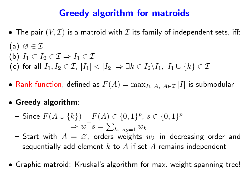
The pair (V, I) is a matroid with I its family of independent sets, i: (a) I (b) I1 I2 I I1 I (c) for all I1, I2 I, |I1| < |I2| k I2\I1, I1 {k} I Rank function, dened as F (A) = maxIA, Greedy algorithm:
AI
|I| is submodular
Since F (A {k}) F (A) {0, 1}p, s {0, 1}p w s = k, sk =1 wk Start with A = , orders weights wk in decreasing order and sequentially add element k to A if set A remains independent
Graphic matroid: Kruskals algorithm for max. weight spanning tree!
44
Submodular functions Links with convexity
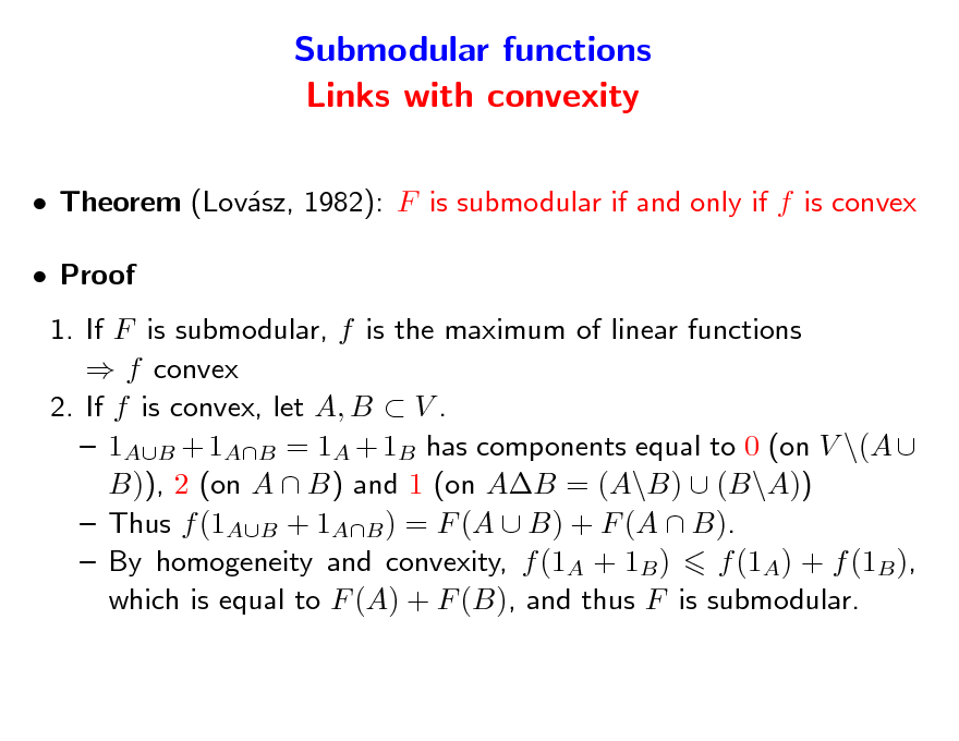
Theorem (Lovsz, 1982): F is submodular if and only if f is convex a Proof 1. If F is submodular, f is the maximum of linear functions f convex 2. If f is convex, let A, B V . 1AB + 1AB = 1A + 1B has components equal to 0 (on V \(A B)), 2 (on A B) and 1 (on AB = (A\B) (B\A)) Thus f (1AB + 1AB ) = F (A B) + F (A B). By homogeneity and convexity, f (1A + 1B ) f (1A) + f (1B ), which is equal to F (A) + F (B), and thus F is submodular.
45
![Slide: Submodular functions Links with convexity
Theorem (Lovsz, 1982): If F is submodular, then a
AV
min F (A) =
w{0,1}p
min
f (w) = min p f (w)
w[0,1]
Proof
1. Since f is an extension of F , minAV F (A) = minw{0,1}p f (w) minw[0,1]p f (w) m 2. Any w [0, 1]p may be decomposed as w = i=1 i1Bi where B1 Bm = V , where 0 and (V ) 1: m m Then f (w) = iF (Bi) i=1 i=1 i minAV F (A) minAV F (A) (because minAV F (A) 0). Thus minw[0,1]p f (w) minAV F (A)](https://yosinski.com/mlss12/media/slides/MLSS-2012-Bach-Learning-with-Submodular-Functions_046.png)
Submodular functions Links with convexity
Theorem (Lovsz, 1982): If F is submodular, then a
AV
min F (A) =
w{0,1}p
min
f (w) = min p f (w)
w[0,1]
Proof
1. Since f is an extension of F , minAV F (A) = minw{0,1}p f (w) minw[0,1]p f (w) m 2. Any w [0, 1]p may be decomposed as w = i=1 i1Bi where B1 Bm = V , where 0 and (V ) 1: m m Then f (w) = iF (Bi) i=1 i=1 i minAV F (A) minAV F (A) (because minAV F (A) 0). Thus minw[0,1]p f (w) minAV F (A)
46
![Slide: Submodular functions Links with convexity
Theorem (Lovsz, 1982): If F is submodular, then a
AV
min F (A) =
w{0,1}p
min
f (w) = min p f (w)
w[0,1]
Consequence: Submodular function minimization may be done in polynomial time Ellipsoid algorithm: polynomial time but slow in practice](https://yosinski.com/mlss12/media/slides/MLSS-2012-Bach-Learning-with-Submodular-Functions_047.png)
Submodular functions Links with convexity
Theorem (Lovsz, 1982): If F is submodular, then a
AV
min F (A) =
w{0,1}p
min
f (w) = min p f (w)
w[0,1]
Consequence: Submodular function minimization may be done in polynomial time Ellipsoid algorithm: polynomial time but slow in practice
47
Submodular functions - Optimization
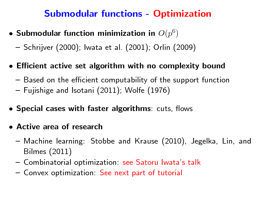
Submodular function minimization in O(p6) Schrijver (2000); Iwata et al. (2001); Orlin (2009) Ecient active set algorithm with no complexity bound Based on the ecient computability of the support function Fujishige and Isotani (2011); Wolfe (1976) Special cases with faster algorithms: cuts, ows Active area of research Machine learning: Stobbe and Krause (2010), Jegelka, Lin, and Bilmes (2011) Combinatorial optimization: see Satoru Iwatas talk Convex optimization: See next part of tutorial
48
Submodular functions - Summary
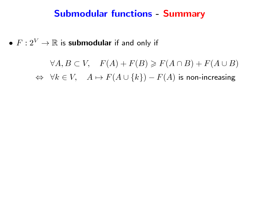
F : 2V R is submodular if and only if k V, A, B V, F (A) + F (B) A F (A {k}) F (A) is non-increasing F (A B) + F (A B)
49
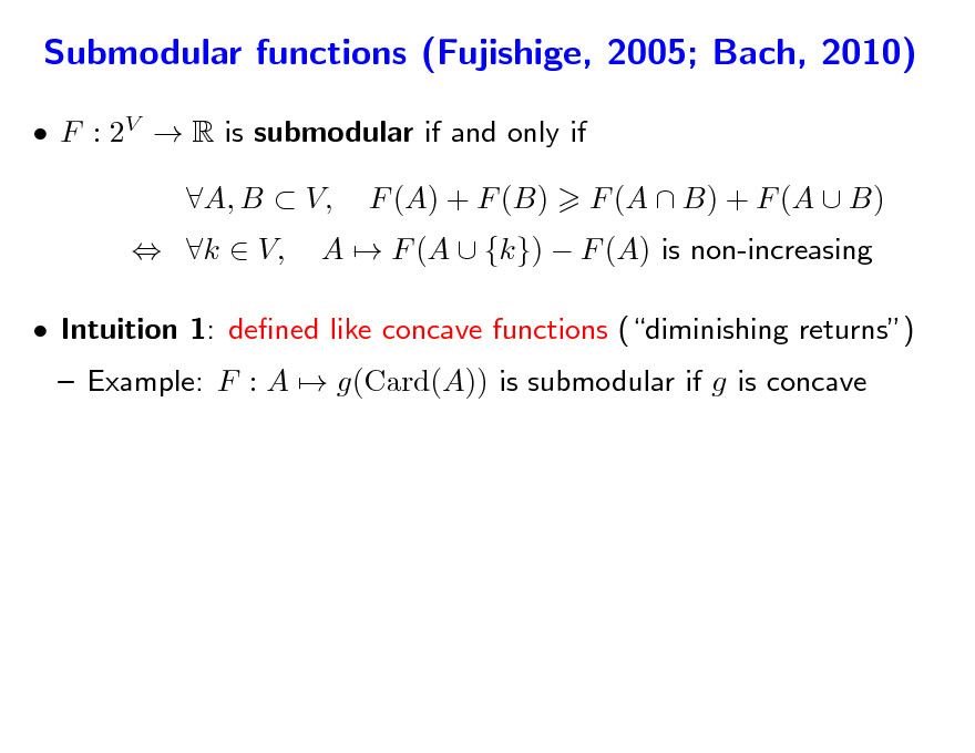
Submodular functions - Summary
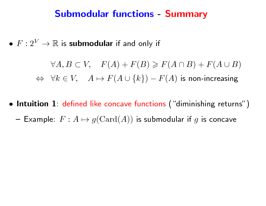
F : 2V R is submodular if and only if k V, A, B V, F (A) + F (B) A F (A {k}) F (A) is non-increasing F (A B) + F (A B)
Intuition 1: dened like concave functions (diminishing returns) Example: F : A g(Card(A)) is submodular if g is concave
50
Submodular functions - Summary
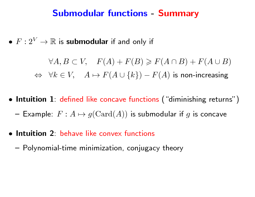
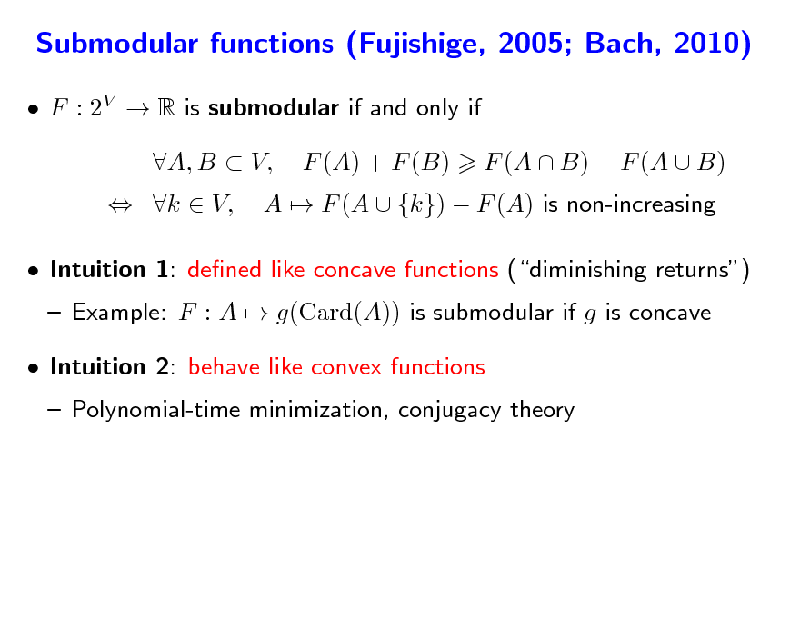
F : 2V R is submodular if and only if k V, A, B V, F (A) + F (B) A F (A {k}) F (A) is non-increasing F (A B) + F (A B)
Intuition 1: dened like concave functions (diminishing returns) Example: F : A g(Card(A)) is submodular if g is concave Intuition 2: behave like convex functions Polynomial-time minimization, conjugacy theory
51
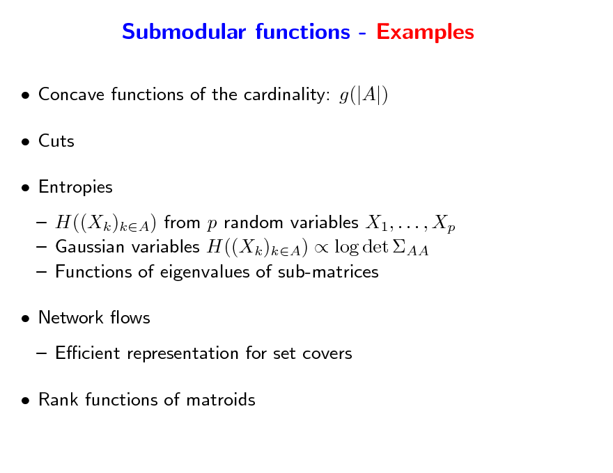
Submodular functions - Examples
Concave functions of the cardinality: g(|A|) Cuts Entropies H((Xk )kA) from p random variables X1, . . . , Xp Gaussian variables H((Xk )kA) log det AA Functions of eigenvalues of sub-matrices Network ows Ecient representation for set covers Rank functions of matroids
52
![Slide: Submodular functions - Lovsz extension a
Given any set-function F and w such that wj1
p
wjp , dene:
f (w) =
k=1 p1
wjk [F ({j1, . . . , jk }) F ({j1, . . . , jk1})]
=
k=1
(wjk wjk+1 )F ({j1, . . . , jk }) + wjp F ({j1, . . . , jp})
If w = 1A, f (w) = F (A) extension from {0, 1}p to Rp (subsets may be identied with elements of {0, 1}p) f is piecewise ane and positively homogeneous F is submodular if and only if f is convex Minimizing f (w) on w [0, 1]p equivalent to minimizing F on 2V](https://yosinski.com/mlss12/media/slides/MLSS-2012-Bach-Learning-with-Submodular-Functions_053.png)
Submodular functions - Lovsz extension a
Given any set-function F and w such that wj1
p
wjp , dene:
f (w) =
k=1 p1
wjk [F ({j1, . . . , jk }) F ({j1, . . . , jk1})]
=
k=1
(wjk wjk+1 )F ({j1, . . . , jk }) + wjp F ({j1, . . . , jp})
If w = 1A, f (w) = F (A) extension from {0, 1}p to Rp (subsets may be identied with elements of {0, 1}p) f is piecewise ane and positively homogeneous F is submodular if and only if f is convex Minimizing f (w) on w [0, 1]p equivalent to minimizing F on 2V
53
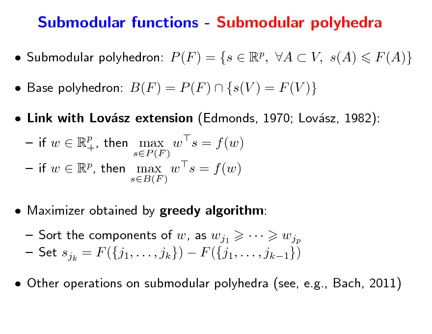
Submodular functions - Submodular polyhedra
Submodular polyhedron: P (F ) = {s Rp, A V, s(A) Base polyhedron: B(F ) = P (F ) {s(V ) = F (V )} Link with Lovsz extension (Edmonds, 1970; Lovsz, 1982): a a if w Rp , then max w s = f (w) +
sP (F ) sB(F )
F (A)}
if w Rp, then max w s = f (w) Maximizer obtained by greedy algorithm: Sort the components of w, as wj1 wjp Set sjk = F ({j1, . . . , jk }) F ({j1, . . . , jk1}) Other operations on submodular polyhedra (see, e.g., Bach, 2011)
54

Outline
1. Submodular functions Denitions Examples of submodular functions Links with convexity through Lovsz extension a 2. Submodular optimization Minimization Links with convex optimization Maximization 3. Structured sparsity-inducing norms Norms with overlapping groups Relaxation of the penalization of supports by submodular functions
55
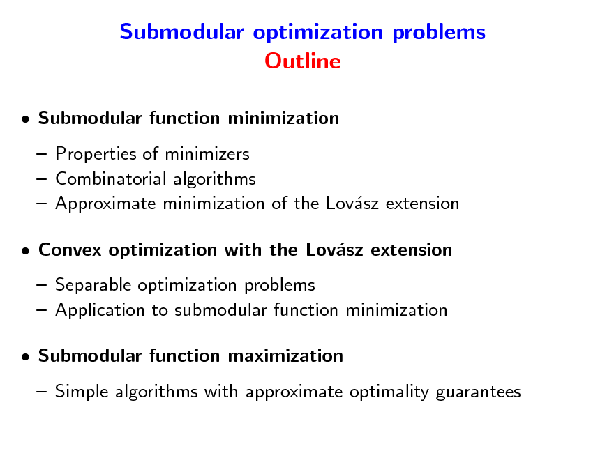
Submodular optimization problems Outline
Submodular function minimization Properties of minimizers Combinatorial algorithms Approximate minimization of the Lovsz extension a Convex optimization with the Lovsz extension a Separable optimization problems Application to submodular function minimization Submodular function maximization Simple algorithms with approximate optimality guarantees
56
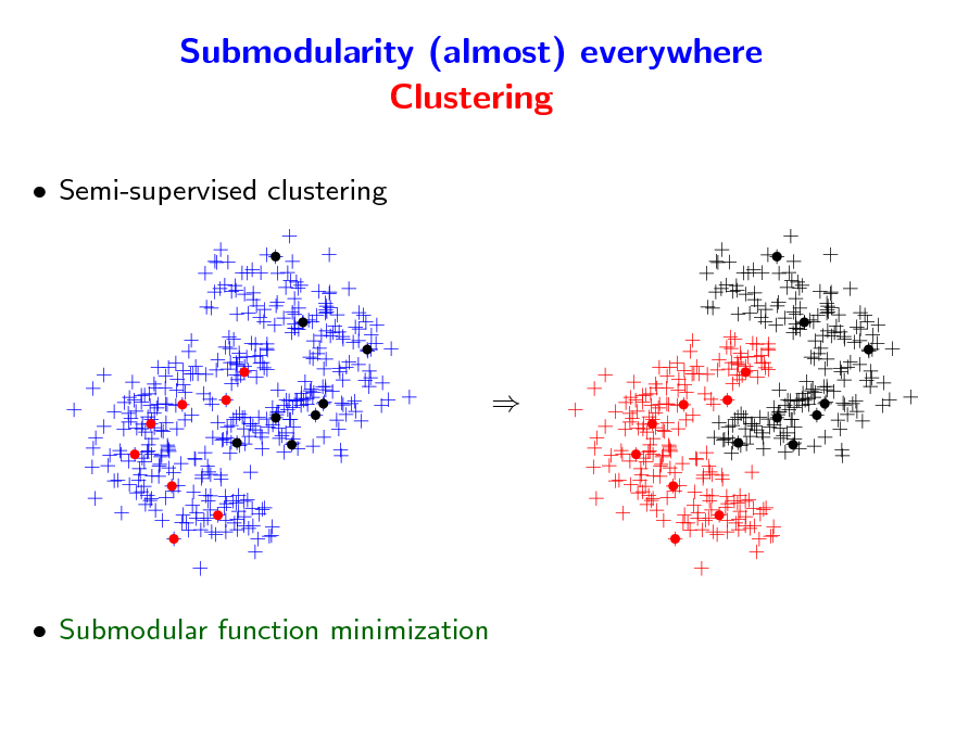
Submodularity (almost) everywhere Clustering
Semi-supervised clustering
Submodular function minimization
57
Submodularity (almost) everywhere Graph cuts
Submodular function minimization
58
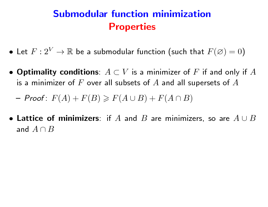
Submodular function minimization Properties
Let F : 2V R be a submodular function (such that F () = 0) Optimality conditions: A V is a minimizer of F if and only if A is a minimizer of F over all subsets of A and all supersets of A Proof : F (A) + F (B) F (A B) + F (A B)
Lattice of minimizers: if A and B are minimizers, so are A B and A B
59
![Slide: Submodular function minimization Dual problem
Let F : 2V R be a submodular function (such that F () = 0) Convex duality:
AV
min F (A) = = =
w[0,1]
min p f (w) min p max w s min p w s = max s(V )
sB(F )
w[0,1] sB(F ) sB(F ) w[0,1]
max
Optimality conditions: The pair (A, s) is optimal if and only if s B(F ) and {s < 0} A {s 0} and s(A) = F (A) Proof : F (A) s(A) = s(A {s < 0}) + s(A {s > 0}) s(A {s < 0}) s(V )](https://yosinski.com/mlss12/media/slides/MLSS-2012-Bach-Learning-with-Submodular-Functions_060.png)
Submodular function minimization Dual problem
Let F : 2V R be a submodular function (such that F () = 0) Convex duality:
AV
min F (A) = = =
w[0,1]
min p f (w) min p max w s min p w s = max s(V )
sB(F )
w[0,1] sB(F ) sB(F ) w[0,1]
max
Optimality conditions: The pair (A, s) is optimal if and only if s B(F ) and {s < 0} A {s 0} and s(A) = F (A) Proof : F (A) s(A) = s(A {s < 0}) + s(A {s > 0}) s(A {s < 0}) s(V )
60
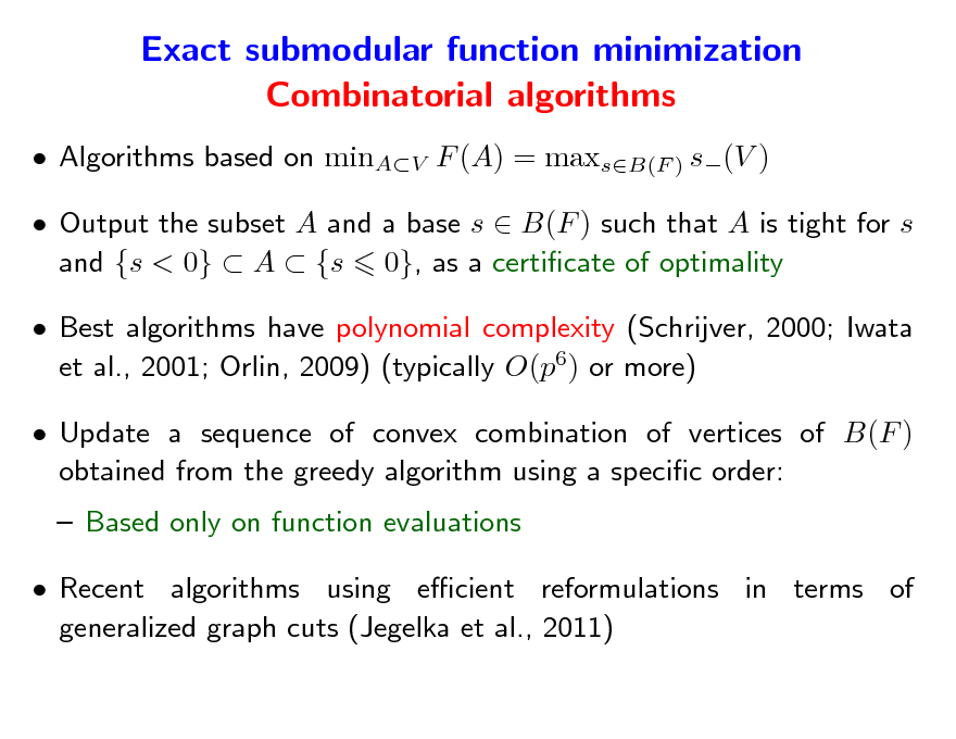
Exact submodular function minimization Combinatorial algorithms
Algorithms based on minAV F (A) = maxsB(F ) s(V ) Output the subset A and a base s B(F ) such that A is tight for s and {s < 0} A {s 0}, as a certicate of optimality Best algorithms have polynomial complexity (Schrijver, 2000; Iwata et al., 2001; Orlin, 2009) (typically O(p6) or more) Update a sequence of convex combination of vertices of B(F ) obtained from the greedy algorithm using a specic order: Based only on function evaluations Recent algorithms using ecient reformulations in terms of generalized graph cuts (Jegelka et al., 2011)
61
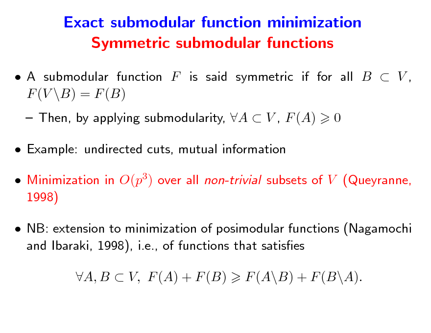
Exact submodular function minimization Symmetric submodular functions
A submodular function F is said symmetric if for all B V , F (V \B) = F (B) Then, by applying submodularity, A V , F (A) Example: undirected cuts, mutual information Minimization in O(p3) over all non-trivial subsets of V (Queyranne, 1998) NB: extension to minimization of posimodular functions (Nagamochi and Ibaraki, 1998), i.e., of functions that satises A, B V, F (A) + F (B) F (A\B) + F (B\A). 0
62
![Slide: Approximate submodular function minimization
For most machine learning applications, no need to obtain exact minimum For convex optimization, see, e.g., Bottou and Bousquet (2008) min F (A) = min f (w) = min p f (w)
w[0,1]
AV
w{0,1}p](https://yosinski.com/mlss12/media/slides/MLSS-2012-Bach-Learning-with-Submodular-Functions_063.png)
Approximate submodular function minimization
For most machine learning applications, no need to obtain exact minimum For convex optimization, see, e.g., Bottou and Bousquet (2008) min F (A) = min f (w) = min p f (w)
w[0,1]
AV
w{0,1}p
63
![Slide: Approximate submodular function minimization
For most machine learning applications, no need to obtain exact minimum For convex optimization, see, e.g., Bottou and Bousquet (2008) min F (A) = min f (w) = min p f (w)
w[0,1]
AV
w{0,1}p
Subgradient of f (w) = max sw through the greedy algorithm
sB(F )
Using projected subgradient descent to minimize f on [0, 1]p
C Iteration: wt = [0,1]p wt1 t st where st f (wt1) C Convergence rate: f (wt)minw[0,1]p f (w) t with primal/dual guarantees (Nesterov, 2003; Bach, 2011)](https://yosinski.com/mlss12/media/slides/MLSS-2012-Bach-Learning-with-Submodular-Functions_064.png)
Approximate submodular function minimization
For most machine learning applications, no need to obtain exact minimum For convex optimization, see, e.g., Bottou and Bousquet (2008) min F (A) = min f (w) = min p f (w)
w[0,1]
AV
w{0,1}p
Subgradient of f (w) = max sw through the greedy algorithm
sB(F )
Using projected subgradient descent to minimize f on [0, 1]p
C Iteration: wt = [0,1]p wt1 t st where st f (wt1) C Convergence rate: f (wt)minw[0,1]p f (w) t with primal/dual guarantees (Nesterov, 2003; Bach, 2011)
64
![Slide: Approximate submodular function minimization Projected subgradient descent
Assume (wlog.) that k V , F ({k}) Denote D2 =
kV
0 and F (V \{k})
F (V )
F ({k}) + F (V \{k}) F (V ) D wt1 st with st argmin wt1s pt sB(F )
Iteration: wt = [0,1]p
Proposition: t iterations of subgradient descent outputs a set At (and a certicate of optimality st) such that F (At) min F (B)
BV
F (At) (st)(V )
Dp1/2 t](https://yosinski.com/mlss12/media/slides/MLSS-2012-Bach-Learning-with-Submodular-Functions_065.png)
Approximate submodular function minimization Projected subgradient descent
Assume (wlog.) that k V , F ({k}) Denote D2 =
kV
0 and F (V \{k})
F (V )
F ({k}) + F (V \{k}) F (V ) D wt1 st with st argmin wt1s pt sB(F )
Iteration: wt = [0,1]p
Proposition: t iterations of subgradient descent outputs a set At (and a certicate of optimality st) such that F (At) min F (B)
BV
F (At) (st)(V )
Dp1/2 t
65

Submodular optimization problems Outline
Submodular function minimization Properties of minimizers Combinatorial algorithms Approximate minimization of the Lovsz extension a Convex optimization with the Lovsz extension a Separable optimization problems Application to submodular function minimization Submodular function maximization Simple algorithms with approximate optimality guarantees
66

Separable optimization on base polyhedron
Optimization of convex functions of the form (w) + f (w) with f Lovsz extension of F a Structured sparsity
Regularized risk minimization penalized by the Lovsz extension a Total variation denoising - isotonic regression
67
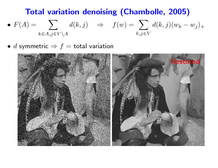
Total variation denoising (Chambolle, 2005)
F (A) = d(k, j)
kA,jV \A
f (w) =
k,jV
d(k, j)(wk wj )+
d symmetric f = total variation
68
Isotonic regression
Given real numbers xi, i = 1, . . . , p
p p
1 Find y R that minimizes (xi yi)2 such that i, yi 2 j=1 y
yi+1
x
For a directed chain, f (y) = 0 if and only if i, yi Minimize
1 2 p j=1(xi
yi+1
yi)2 + f (y) for large
69
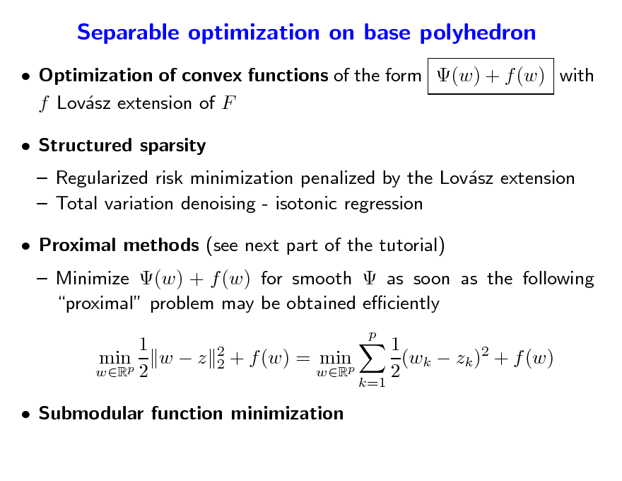
Separable optimization on base polyhedron
Optimization of convex functions of the form (w) + f (w) with f Lovsz extension of F a Structured sparsity
Regularized risk minimization penalized by the Lovsz extension a Total variation denoising - isotonic regression
70
Separable optimization on base polyhedron
Optimization of convex functions of the form (w) + f (w) with f Lovsz extension of F a Structured sparsity
Regularized risk minimization penalized by the Lovsz extension a Total variation denoising - isotonic regression
Proximal methods (see next part of the tutorial)
Minimize (w) + f (w) for smooth as soon as the following proximal problem may be obtained eciently 1 minp w z wR 2
p 2 2
+ f (w) = minp
wR k=1
1 (wk zk )2 + f (w) 2
Submodular function minimization
71
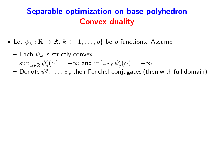
Separable optimization on base polyhedron Convex duality
Let k : R R, k {1, . . . , p} be p functions. Assume Each k is strictly convex supR j () = + and inf R j () = Denote 1 , . . . , p their Fenchel-conjugates (then with full domain)
72
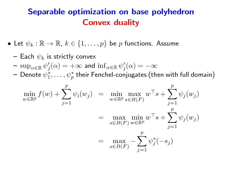
Separable optimization on base polyhedron Convex duality
Let k : R R, k {1, . . . , p} be p functions. Assume Each k is strictly convex supR j () = + and inf R j () = Denote 1 , . . . , p their Fenchel-conjugates (then with full domain)
p wR p
minp f (w) +
j=1
i(wj ) = minp max w s +
wR sB(F ) j=1 p
j (wj ) j (wj )
j=1
= =
sB(F ) wR
max minp w s +
p j (sj ) j=1
sB(F )
max
73
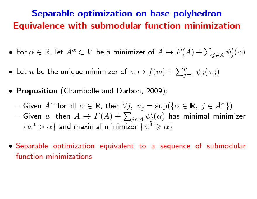
Separable optimization on base polyhedron Equivalence with submodular function minimization
For R, let A V be a minimizer of A F (A) + Let u be the unique minimizer of w f (w) + Proposition (Chambolle and Darbon, 2009): Given A for all R, then j, uj = sup({ R, j A}) Given u, then A F (A) + jA j () has minimal minimizer {w > } and maximal minimizer {w } Separable optimization equivalent to a sequence of submodular function minimizations
j () jA
p j=1 j (wj )
74
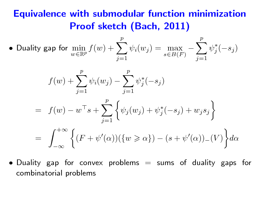
Equivalence with submodular function minimization Proof sketch (Bach, 2011)
p p
Duality gap for minp f (w) +
wR p
j=1
i(wj ) = max
sB(F ) j (sj )
j (sj ) j=1
p
f (w) +
j=1
i(wj )
p
j=1
= f (w) w s +
+
j (wj ) + j (sj ) + wj sj j=1
=
(F + ())({w
}) (s + ())(V ) d
Duality gap for convex problems = sums of duality gaps for combinatorial problems
75
Separable optimization on base polyhedron Quadratic case
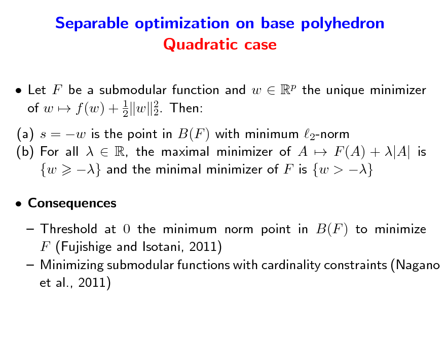
Let F be a submodular function and w Rp the unique minimizer of w f (w) + 1 w 2. Then: 2 2 (a) s = w is the point in B(F ) with minimum 2-norm (b) For all R, the maximal minimizer of A F (A) + |A| is {w } and the minimal minimizer of F is {w > } Consequences Threshold at 0 the minimum norm point in B(F ) to minimize F (Fujishige and Isotani, 2011) Minimizing submodular functions with cardinality constraints (Nagano et al., 2011)
76
From convex to combinatorial optimization and vice-versa...
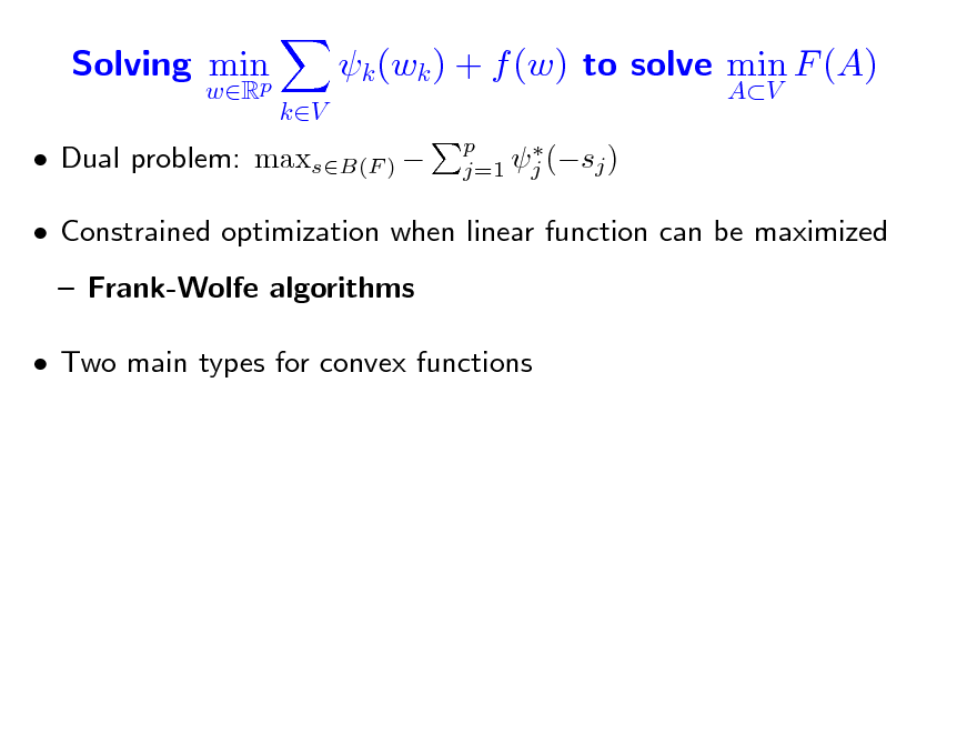
Solving minp
wR
k (wk ) + f (w) to solve min F (A)
kV AV
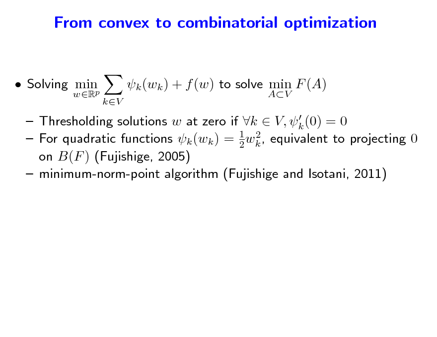
Thresholding solutions w at zero if k V, k (0) = 0 2 For quadratic functions k (wk ) = 1 wk , equivalent to projecting 0 2 on B(F ) (Fujishige, 2005) minimum-norm-point algorithm (Fujishige and Isotani, 2011)
77
From convex to combinatorial optimization and vice-versa...
Solving minp
wR
k (wk ) + f (w) to solve min F (A)
kV AV
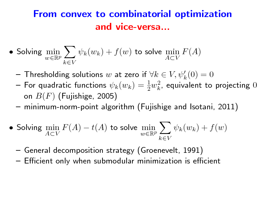
Thresholding solutions w at zero if k V, k (0) = 0 2 For quadratic functions k (wk ) = 1 wk , equivalent to projecting 0 2 on B(F ) (Fujishige, 2005) minimum-norm-point algorithm (Fujishige and Isotani, 2011)
Solving min F (A) t(A) to solve minp
AV wR
k (wk ) + f (w)
kV
General decomposition strategy (Groenevelt, 1991) Ecient only when submodular minimization is ecient
78
Solving min F (A) t(A) to solve min p
AV wR
k (wk )+f (w)
kV
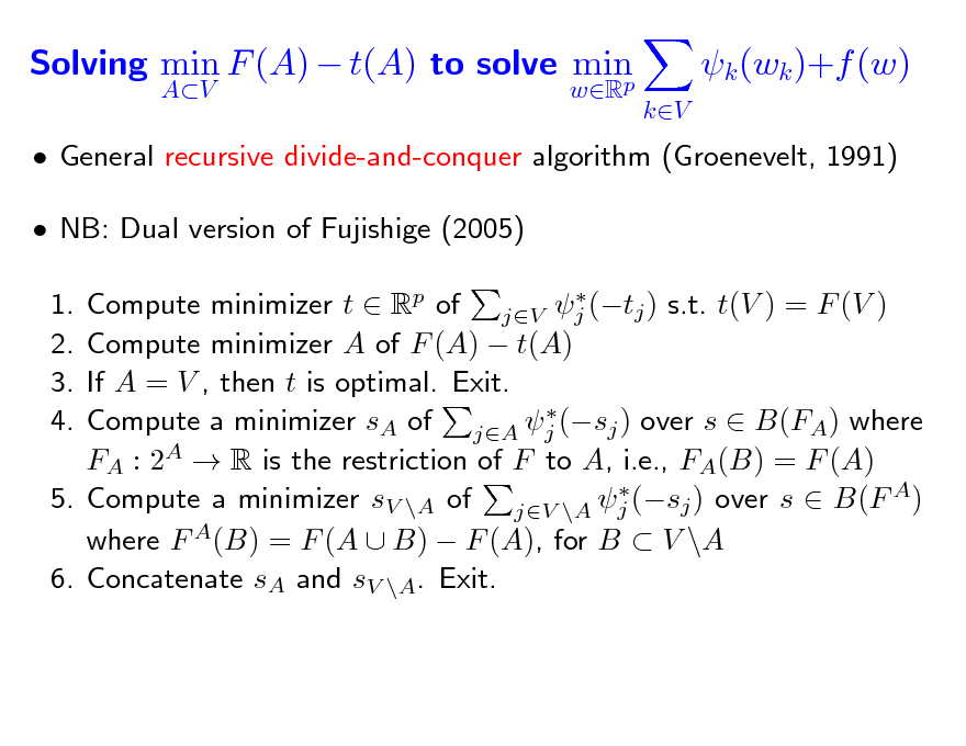
General recursive divide-and-conquer algorithm (Groenevelt, 1991) NB: Dual version of Fujishige (2005)
Compute minimizer t Rp of jV j (tj ) s.t. t(V ) = F (V ) Compute minimizer A of F (A) t(A) If A = V , then t is optimal. Exit. Compute a minimizer sA of jA j (sj ) over s B(FA) where FA : 2A R is the restriction of F to A, i.e., FA(B) = F (A) 5. Compute a minimizer sV \A of jV \A j (sj ) over s B(F A) where F A(B) = F (A B) F (A), for B V \A 6. Concatenate sA and sV \A. Exit.
1. 2. 3. 4.
79
Solving min p
wR kV
k (wk ) + f (w) to solve min F (A)
AV
p j (sj ) j=1
Dual problem: maxsB(F )
Constrained optimization when linear function can be maximized Frank-Wolfe algorithms Two main types for convex functions
80
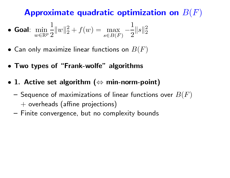
Approximate quadratic optimization on B(F )
1 Goal: minp w wR 2
2 2
1 + f (w) = max s sB(F ) 2
2 2
Can only maximize linear functions on B(F ) Two types of Frank-wolfe algorithms 1. Active set algorithm ( min-norm-point) Sequence of maximizations of linear functions over B(F ) + overheads (ane projections) Finite convergence, but no complexity bounds
81
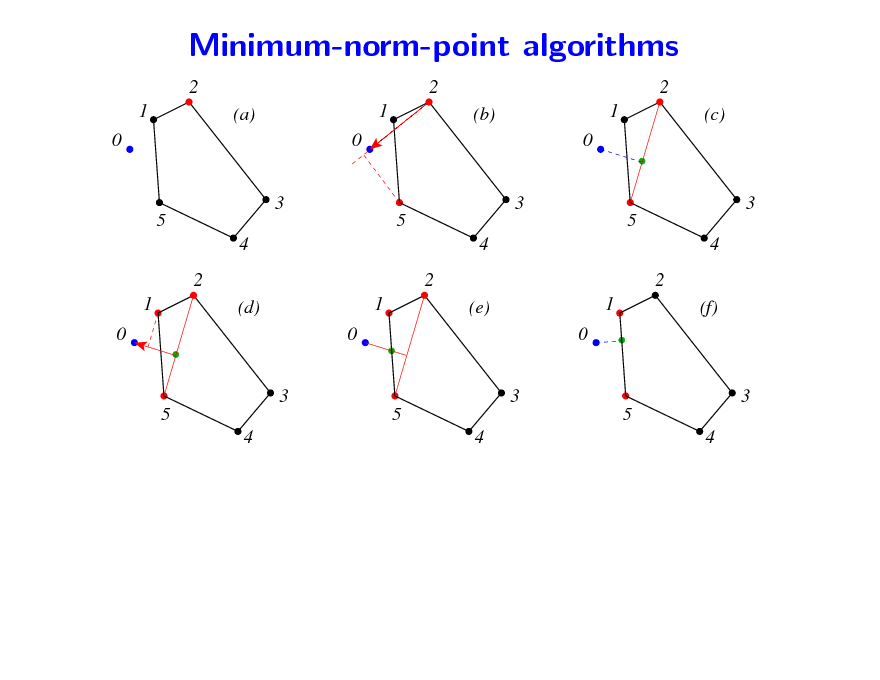
Minimum-norm-point algorithms
2 1 0 3 5 4 2 1 0 3 5 4 5 4 (d) 0 3 5 4 1 2 (e) 0 3 1 5 4 2 (f) (a) 0 3 5 4 1 2 (b) 0 3 1 2 (c)
82
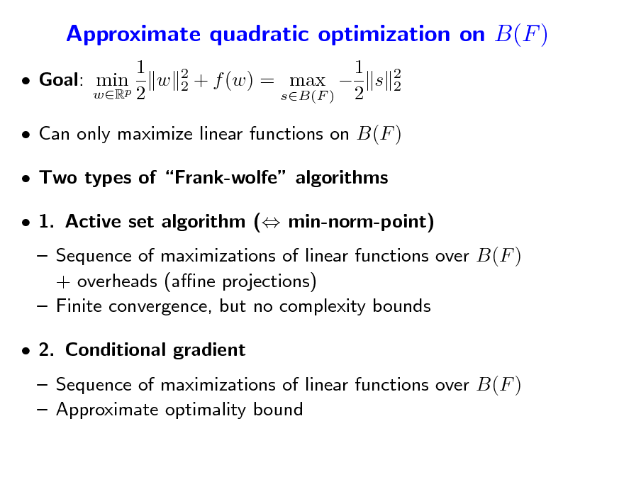
Approximate quadratic optimization on B(F )
1 Goal: minp w wR 2
2 2
1 + f (w) = max s sB(F ) 2
2 2
Can only maximize linear functions on B(F ) Two types of Frank-wolfe algorithms 1. Active set algorithm ( min-norm-point) Sequence of maximizations of linear functions over B(F ) + overheads (ane projections) Finite convergence, but no complexity bounds 2. Conditional gradient Sequence of maximizations of linear functions over B(F ) Approximate optimality bound
83
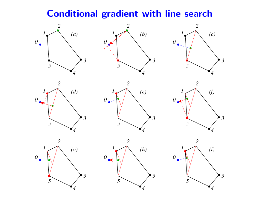
Conditional gradient with line search
2 1 0 3 5 4 2 1 0 3 5 4 2 1 0 3 5 4 5 4 (g) 0 3 5 4 1 2 (h) 0 3 1 5 4 2 (i) (d) 0 3 5 4 1 2 (e) 0 3 1 5 4 2 (f) (a) 0 3 5 4 1 2 (b) 0 3 1 2 (c)
84
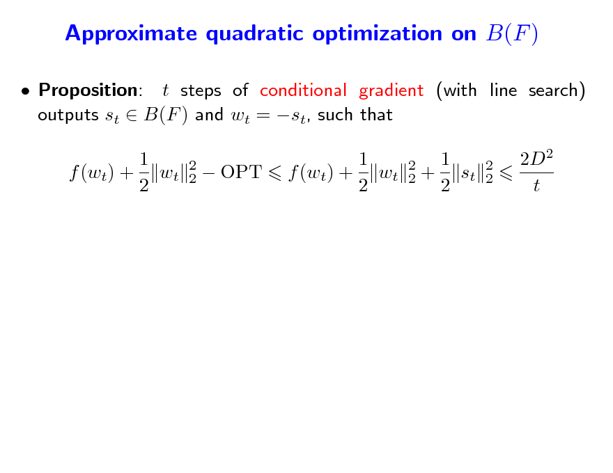
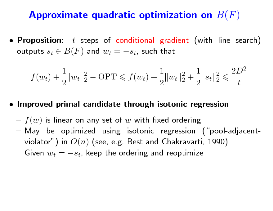
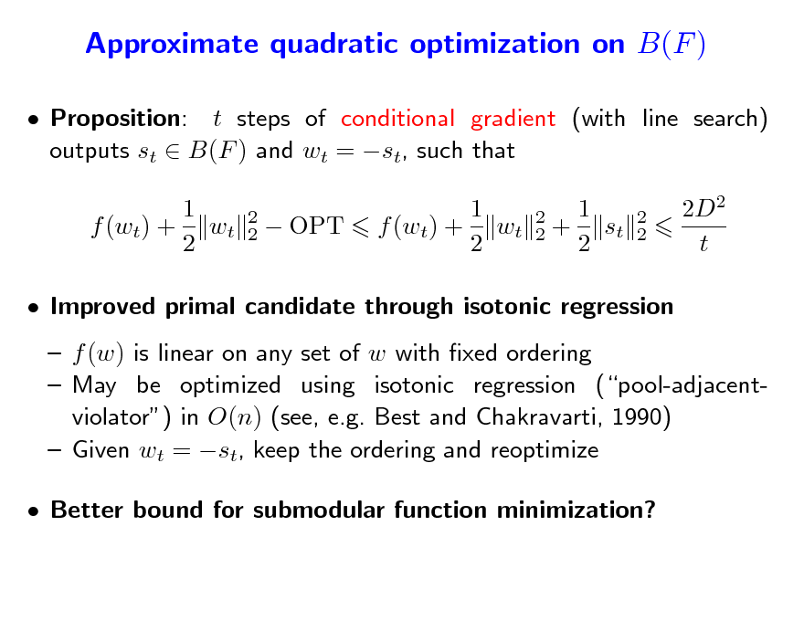
Approximate quadratic optimization on B(F )
Proposition: t steps of conditional gradient (with line search) outputs st B(F ) and wt = st, such that 1 f (wt) + wt 2
2 2
OPT
1 f (wt) + wt 2
2 2
1 + st 2
2 2
2D2 t
85
Approximate quadratic optimization on B(F )
Proposition: t steps of conditional gradient (with line search) outputs st B(F ) and wt = st, such that 1 f (wt) + wt 2
2 2
OPT
1 f (wt) + wt 2
2 2
1 + st 2
2 2
2D2 t
Improved primal candidate through isotonic regression f (w) is linear on any set of w with xed ordering May be optimized using isotonic regression (pool-adjacentviolator) in O(n) (see, e.g. Best and Chakravarti, 1990) Given wt = st, keep the ordering and reoptimize
86
Approximate quadratic optimization on B(F )
Proposition: t steps of conditional gradient (with line search) outputs st B(F ) and wt = st, such that 1 f (wt) + wt 2
2 2
OPT
1 f (wt) + wt 2
2 2
1 + st 2
2 2
2D2 t
Improved primal candidate through isotonic regression f (w) is linear on any set of w with xed ordering May be optimized using isotonic regression (pool-adjacentviolator) in O(n) (see, e.g. Best and Chakravarti, 1990) Given wt = st, keep the ordering and reoptimize Better bound for submodular function minimization?
87
From quadratic optimization on B(F ) to submodular function minimization
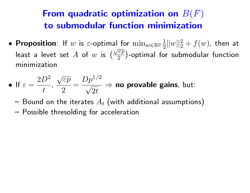
Proposition: If w is -optimal for minwRp 1 w 2 + f (w), then at 2 2 p least a levet set A of w is 2 -optimal for submodular function minimization 2 p 2D Dp1/2 If = , = no provable gains, but: t 2 2t Bound on the iterates At (with additional assumptions) Possible thresolding for acceleration
88
From quadratic optimization on B(F ) to submodular function minimization
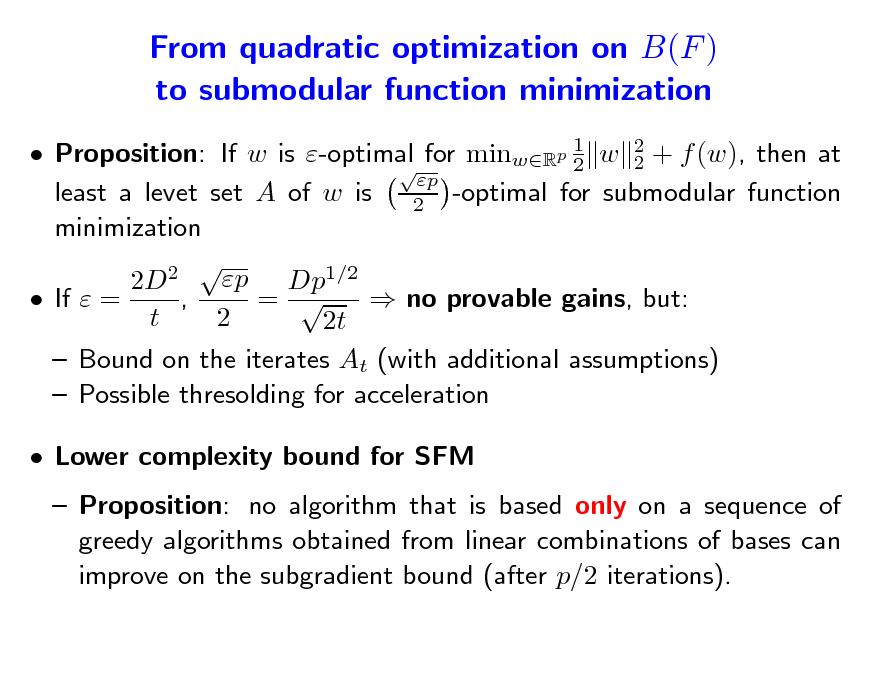
Proposition: If w is -optimal for minwRp 1 w 2 + f (w), then at 2 2 p least a levet set A of w is 2 -optimal for submodular function minimization 2 p Dp1/2 2D , = If = no provable gains, but: t 2 2t Bound on the iterates At (with additional assumptions) Possible thresolding for acceleration Lower complexity bound for SFM Proposition: no algorithm that is based only on a sequence of greedy algorithms obtained from linear combinations of bases can improve on the subgradient bound (after p/2 iterations).
89
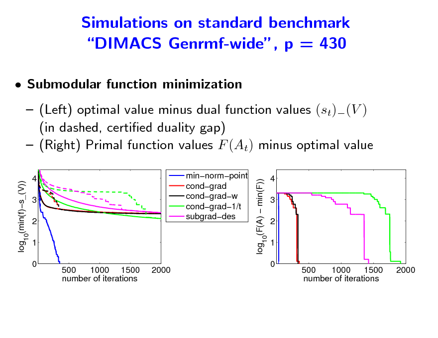
Simulations on standard benchmark DIMACS Genrmf-wide, p = 430
Submodular function minimization (Left) optimal value minus dual function values (st)(V ) (in dashed, certied duality gap) (Right) Primal function values F (At) minus optimal value
log10(F(A) min(F))
log10(min(f)s_(V)) 4 3 2 1 0 500 1000 1500 number of iterations 2000 minnormpoint condgrad condgradw condgrad1/t subgraddes
4 3 2 1 0 500 1000 1500 number of iterations 2000
90
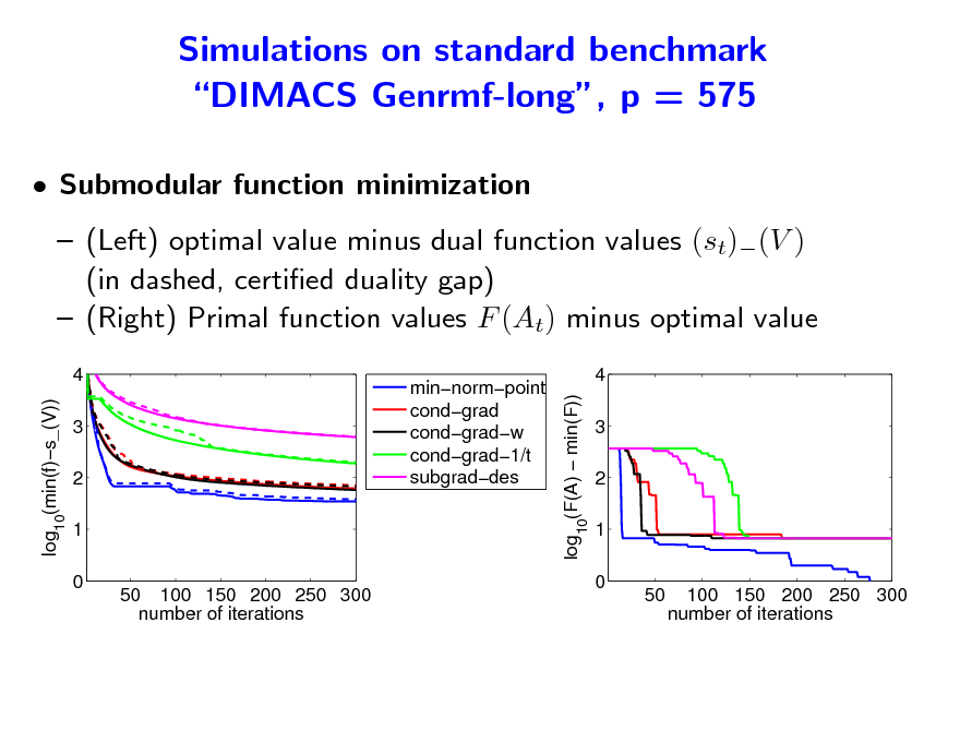
Simulations on standard benchmark DIMACS Genrmf-long, p = 575
Submodular function minimization (Left) optimal value minus dual function values (st)(V ) (in dashed, certied duality gap) (Right) Primal function values F (At) minus optimal value
4 log (min(f)s_(V)) 3 2 1 0
log (F(A) min(F))
minnormpoint condgrad condgradw condgrad1/t subgraddes
4 3 2 1 0
10
10
50 100 150 200 250 300 number of iterations
50
100 150 200 250 300 number of iterations
91
Simulations on standard benchmark
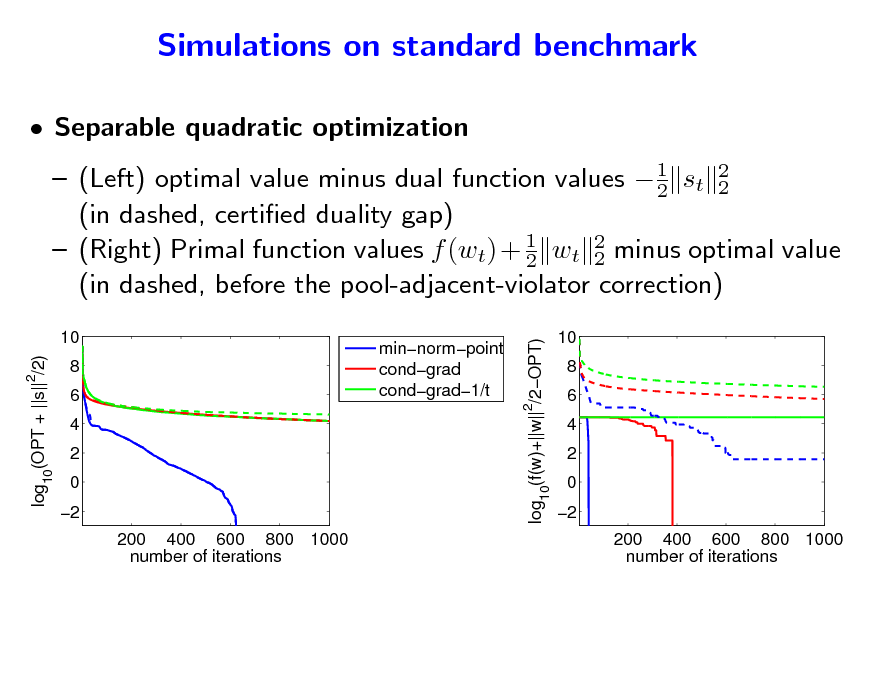
Separable quadratic optimization
1 (Left) optimal value minus dual function values 2 st 2 2 (in dashed, certied duality gap) (Right) Primal function values f (wt) + 1 wt 2 minus optimal value 2 2 (in dashed, before the pool-adjacent-violator correction)
minnormpoint condgrad condgrad1/t
log10(f(w)+||w||2/2OPT)
10 log10(OPT + ||s|| /2)
2
10 8 6 4 2 0 2 200 400 600 800 1000 number of iterations
8 6 4 2 0 2 200 400 600 800 1000 number of iterations
92

Submodularity (almost) everywhere Sensor placement
Each sensor covers a certain area (Krause and Guestrin, 2005) Goal: maximize coverage
Submodular function maximization Extension to experimental design (Seeger, 2009)
93
Submodular function maximization
Occurs in various form in applications but is NP-hard Unconstrained maximization: Feige et al. (2007) shows that that for non-negative functions, a random subset already achieves at least 1/4 of the optimal value, while local search techniques achieve at least 1/2 Maximizing non-decreasing cardinality constraint submodular functions with
Greedy algorithm achieves (1 1/e) of the optimal value Proof (Nemhauser et al., 1978)
94
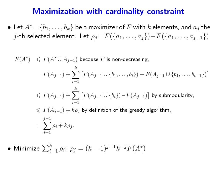
Maximization with cardinality constraint
Let A = {b1, . . . , bk } be a maximizer of F with k elements, and aj the j-th selected element. Let j = F ({a1, . . . , aj })F ({a1, . . . , aj1})
F (A) F (A Aj1 ) because F is non-decreasing,
k
= F (Aj1) +
i=1 k
F (Aj1 {b1, . . . , bi}) F (Aj1 {b1, . . . , bi1}) F (Aj1 {bi})F (Aj1) by submodularity,
F (Aj1) +
i=1
F (Aj1) + kj by denition of the greedy algorithm,
j1
=
i=1
i + kj .
Minimize
k i=1 i:
j = (k 1)j1k j F (A)
95
Submodular optimization problems Summary
Submodular function minimization Properties of minimizers Combinatorial algorithms Approximate minimization of the Lovsz extension a Convex optimization with the Lovsz extension a Separable optimization problems Application to submodular function minimization Submodular function maximization Simple algorithms with approximate optimality guarantees
96

Outline
1. Submodular functions Denitions Examples of submodular functions Links with convexity through Lovsz extension a 2. Submodular optimization Minimization Links with convex optimization Maximization 3. Structured sparsity-inducing norms Norms with overlapping groups Relaxation of the penalization of supports by submodular functions
97
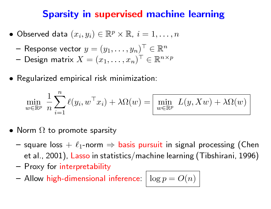
Sparsity in supervised machine learning
Observed data (xi, yi) Rp R, i = 1, . . . , n Response vector y = (y1, . . . , yn) Rn Design matrix X = (x1, . . . , xn) Rnp
n
Regularized empirical risk minimization: 1 minp (yi, w xi) + (w) = minp L(y, Xw) + (w) wR n wR i=1 Norm to promote sparsity
square loss + 1-norm basis pursuit in signal processing (Chen et al., 2001), Lasso in statistics/machine learning (Tibshirani, 1996) Proxy for interpretability Allow high-dimensional inference: log p = O(n)
98
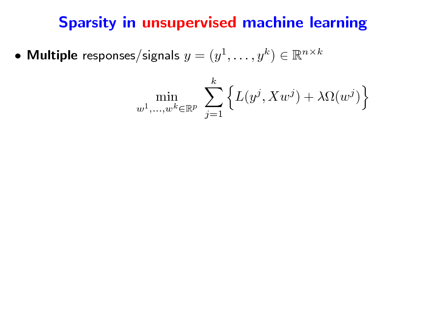
Sparsity in unsupervised machine learning
Multiple responses/signals y = (y 1, . . . , y k ) Rnk
k X=(x1 ,...,xp) w1 ,...,wk Rp
min
min
L(y j , Xw j ) + (w j )
j=1
99
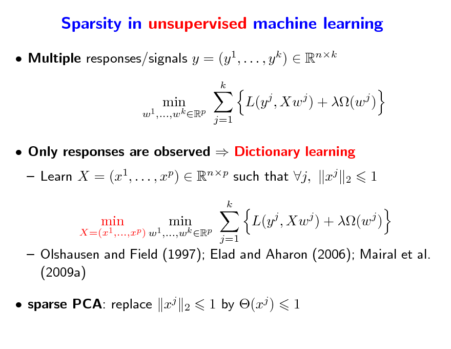
Sparsity in unsupervised machine learning
Multiple responses/signals y = (y 1, . . . , y k ) Rnk
k X=(x1 ,...,xp) w1 ,...,wk Rp
min
min
L(y j , Xw j ) + (w j )
j=1
Only responses are observed Dictionary learning Learn X = (x1, . . . , xp) Rnp such that j, xj
k X=(x1 ,...,xp ) w1 ,...,wk Rp 2
1
min
min
L(y j , Xw j ) + (w j )
j=1
Olshausen and Field (1997); Elad and Aharon (2006); Mairal et al. (2009a) sparse PCA: replace xj
2
1 by (xj )
1
100
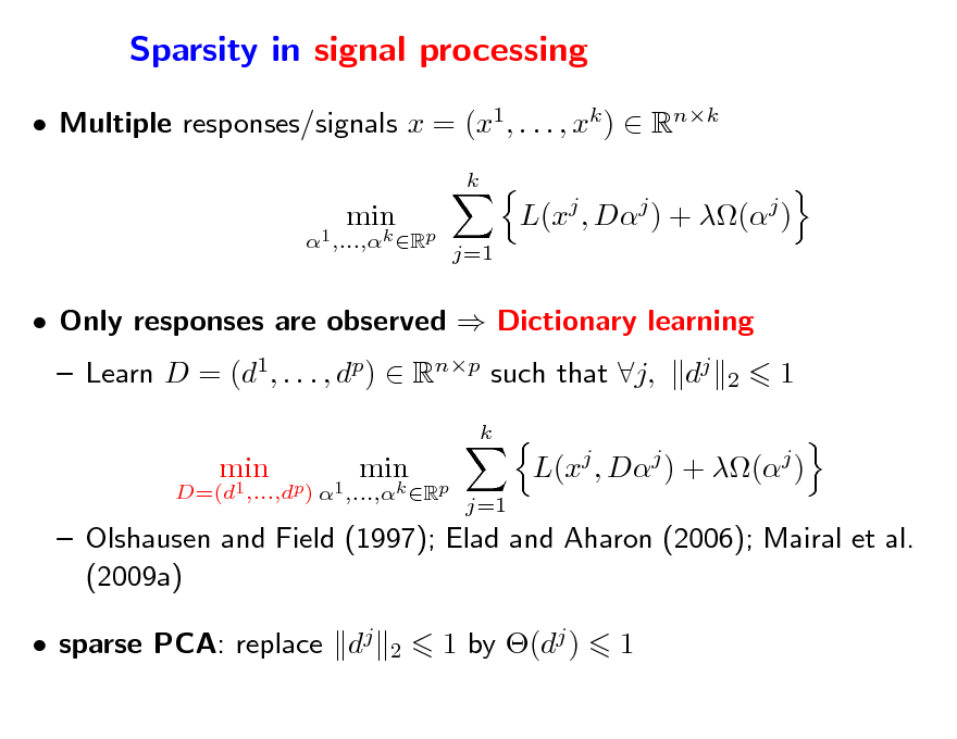
Sparsity in signal processing
Multiple responses/signals x = (x1, . . . , xk ) Rnk
k D=(d1,...,dp) 1 ,...,k Rp
min
min
L(xj , Dj ) + (j )
j=1
Only responses are observed Dictionary learning Learn D = (d1, . . . , dp) Rnp such that j,
k D=(d1 ,...,dp) 1 ,...,k Rp
dj
2
1
min
min
L(xj , Dj ) + (j )
j=1
Olshausen and Field (1997); Elad and Aharon (2006); Mairal et al. (2009a) sparse PCA: replace dj
2
1 by (dj )
1
101

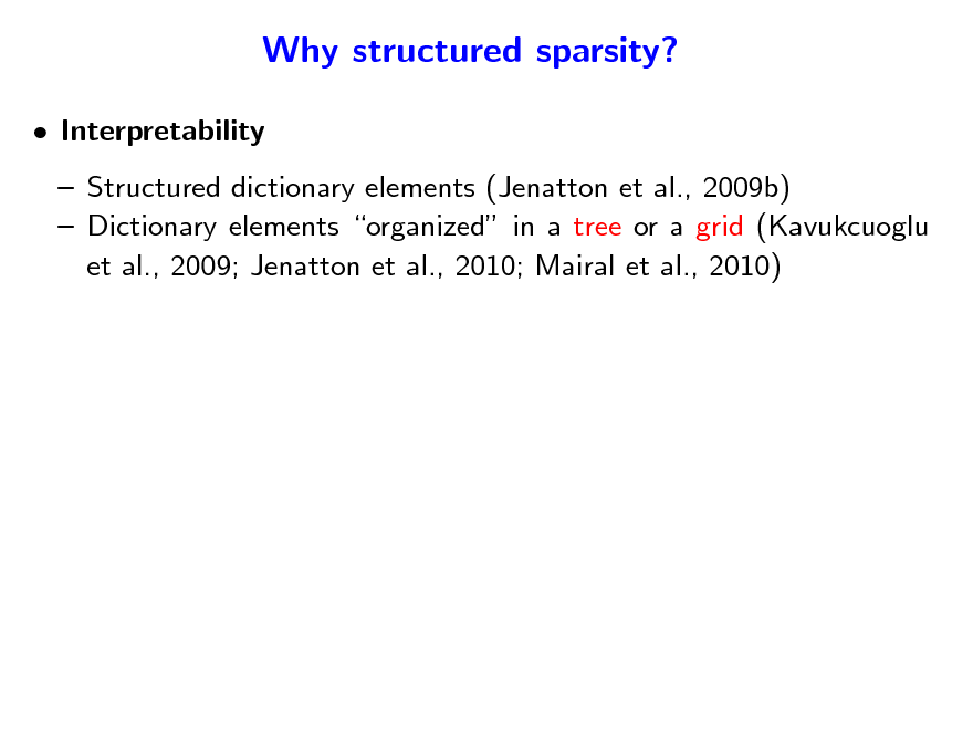
Why structured sparsity?
Interpretability Structured dictionary elements (Jenatton et al., 2009b) Dictionary elements organized in a tree or a grid (Kavukcuoglu et al., 2009; Jenatton et al., 2010; Mairal et al., 2010)
102
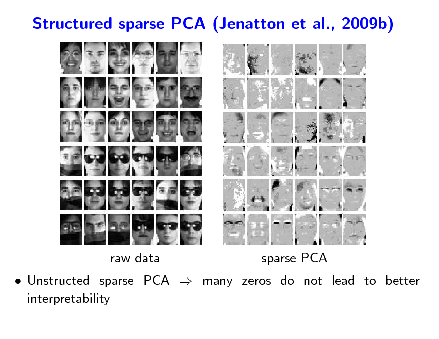
Structured sparse PCA (Jenatton et al., 2009b)
raw data
sparse PCA
Unstructed sparse PCA many zeros do not lead to better interpretability
103
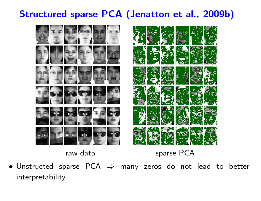
Structured sparse PCA (Jenatton et al., 2009b)
raw data
sparse PCA
Unstructed sparse PCA many zeros do not lead to better interpretability
104
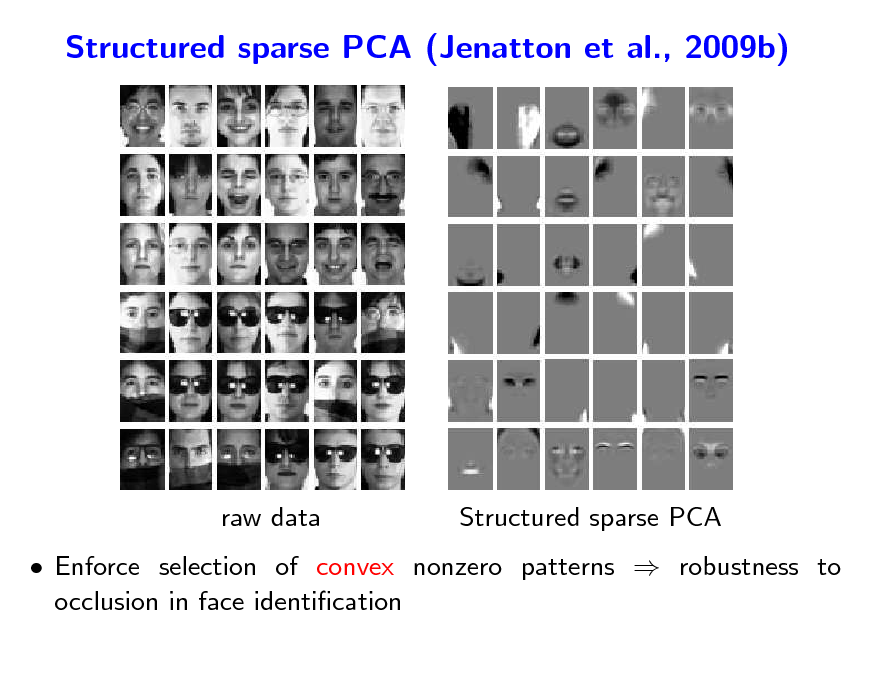
Structured sparse PCA (Jenatton et al., 2009b)
raw data
Structured sparse PCA
Enforce selection of convex nonzero patterns robustness to occlusion in face identication
105
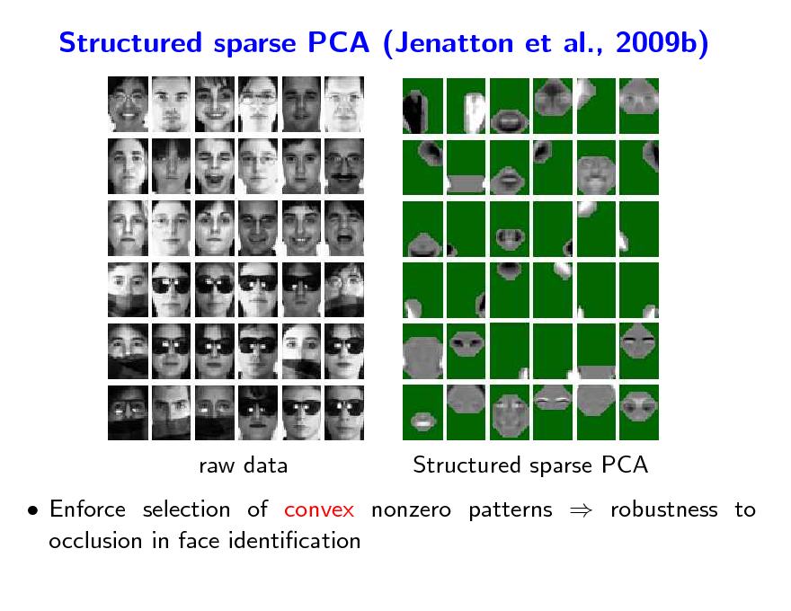
Structured sparse PCA (Jenatton et al., 2009b)
raw data
Structured sparse PCA
Enforce selection of convex nonzero patterns robustness to occlusion in face identication
106

Why structured sparsity?
Interpretability Structured dictionary elements (Jenatton et al., 2009b) Dictionary elements organized in a tree or a grid (Kavukcuoglu et al., 2009; Jenatton et al., 2010; Mairal et al., 2010)
107
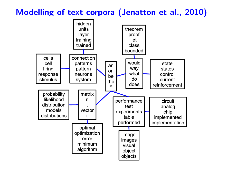
Modelling of text corpora (Jenatton et al., 2010)
108
Why structured sparsity?
Interpretability Structured dictionary elements (Jenatton et al., 2009b) Dictionary elements organized in a tree or a grid (Kavukcuoglu et al., 2009; Jenatton et al., 2010; Mairal et al., 2010)
109
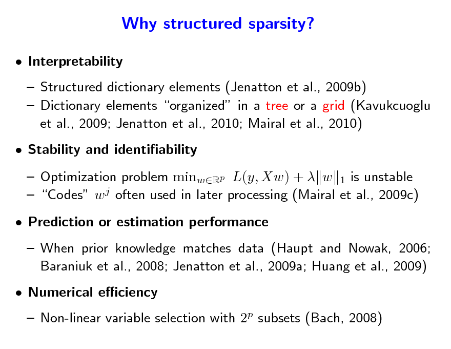
Why structured sparsity?
Interpretability Structured dictionary elements (Jenatton et al., 2009b) Dictionary elements organized in a tree or a grid (Kavukcuoglu et al., 2009; Jenatton et al., 2010; Mairal et al., 2010) Stability and identiability Optimization problem minwRp L(y, Xw) + w 1 is unstable Codes w j often used in later processing (Mairal et al., 2009c) Prediction or estimation performance When prior knowledge matches data (Haupt and Nowak, 2006; Baraniuk et al., 2008; Jenatton et al., 2009a; Huang et al., 2009) Numerical eciency
Non-linear variable selection with 2p subsets (Bach, 2008)
110
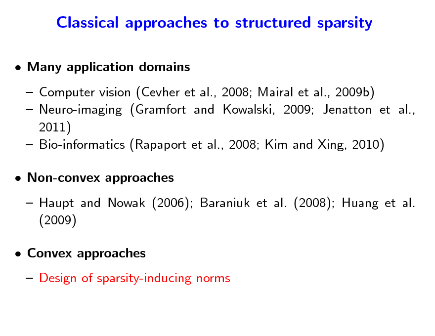
Classical approaches to structured sparsity
Many application domains Computer vision (Cevher et al., 2008; Mairal et al., 2009b) Neuro-imaging (Gramfort and Kowalski, 2009; Jenatton et al., 2011) Bio-informatics (Rapaport et al., 2008; Kim and Xing, 2010) Non-convex approaches Haupt and Nowak (2006); Baraniuk et al. (2008); Huang et al. (2009) Convex approaches Design of sparsity-inducing norms
111
Sparsity-inducing norms
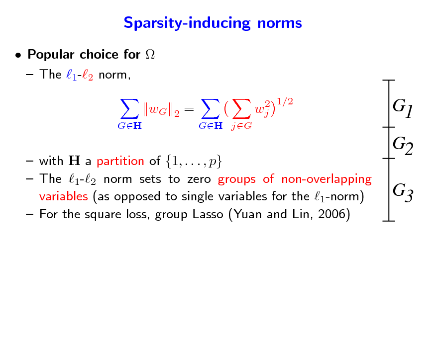
Popular choice for The 1-2 norm, wG
GH 2 = GH jG 2 wj 1/2
G1 G2 G3
with H a partition of {1, . . . , p} The 1-2 norm sets to zero groups of non-overlapping variables (as opposed to single variables for the 1-norm) For the square loss, group Lasso (Yuan and Lin, 2006)
112
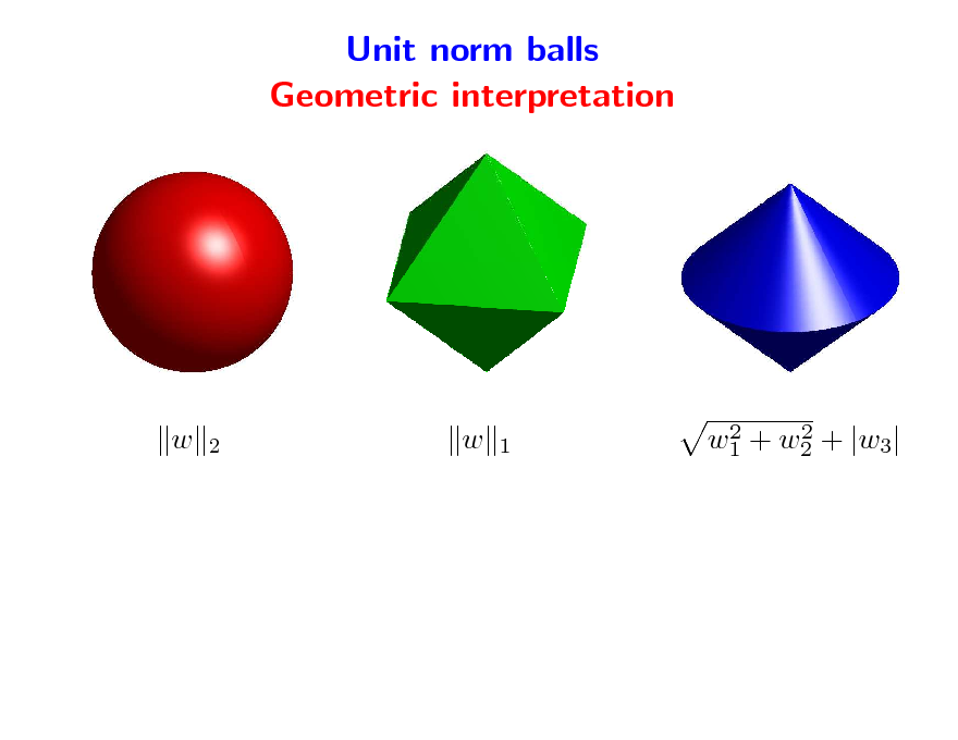
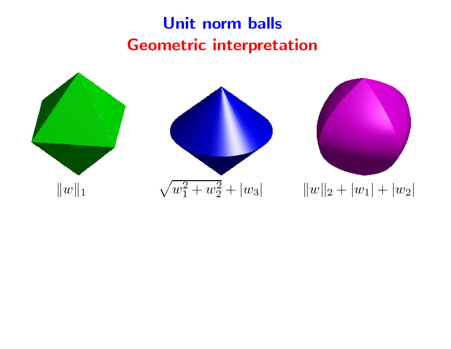
Unit norm balls Geometric interpretation
w
2
w
1
2 2 w1 + w2 + |w3|
113
Sparsity-inducing norms
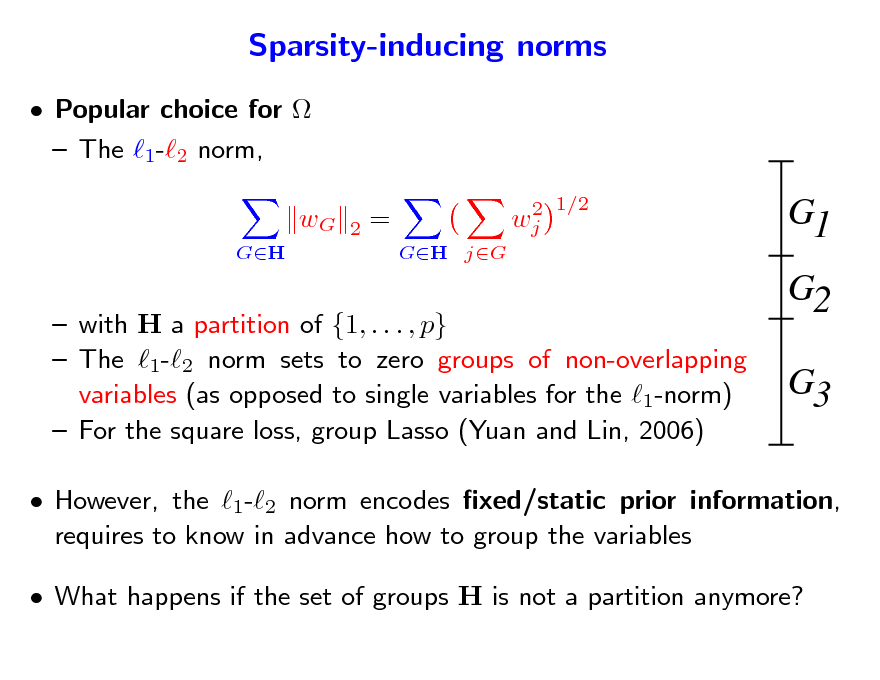
Popular choice for The 1-2 norm, wG
GH 2 = GH jG 2 wj 1/2
G1 G2 G3
with H a partition of {1, . . . , p} The 1-2 norm sets to zero groups of non-overlapping variables (as opposed to single variables for the 1-norm) For the square loss, group Lasso (Yuan and Lin, 2006)
However, the 1-2 norm encodes xed/static prior information, requires to know in advance how to group the variables What happens if the set of groups H is not a partition anymore?
114
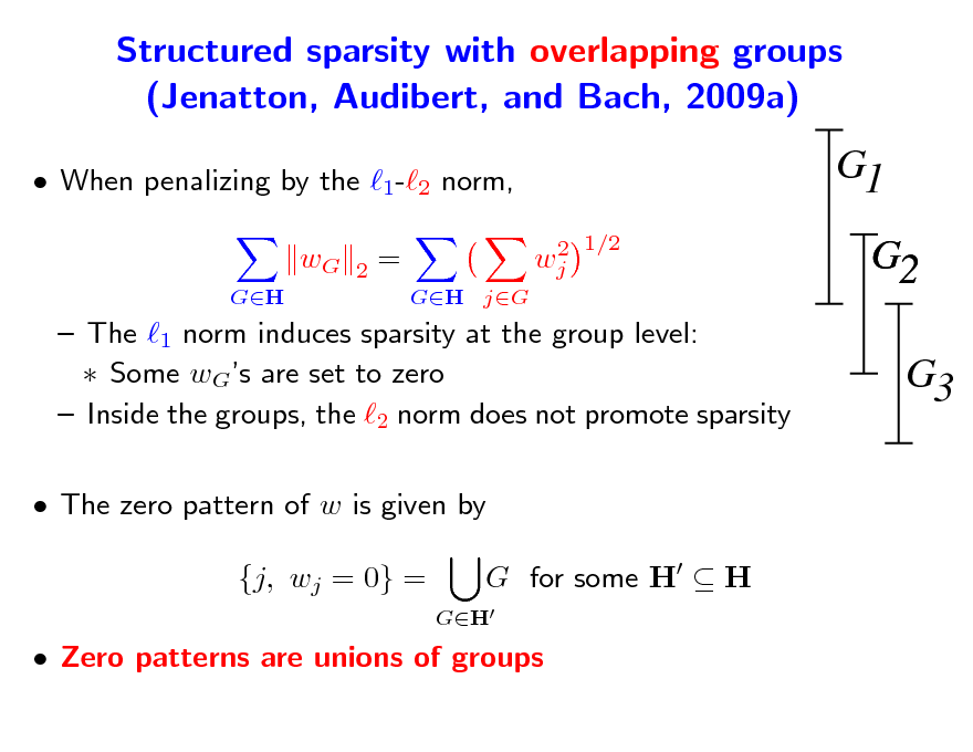
Structured sparsity with overlapping groups (Jenatton, Audibert, and Bach, 2009a)
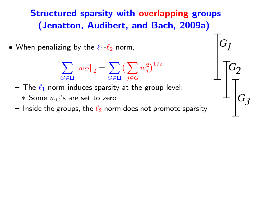
When penalizing by the 1-2 norm, wG
GH 2
G1
2 1/2 wj
=
GH jG
G2 G3
The 1 norm induces sparsity at the group level: Some wGs are set to zero Inside the groups, the 2 norm does not promote sparsity
115
Structured sparsity with overlapping groups (Jenatton, Audibert, and Bach, 2009a)
When penalizing by the 1-2 norm, wG
GH 2
G1
2 1/2 wj
=
GH jG
G2 G3
The 1 norm induces sparsity at the group level: Some wGs are set to zero Inside the groups, the 2 norm does not promote sparsity The zero pattern of w is given by {j, wj = 0} =
GH
G for some H H
Zero patterns are unions of groups
116
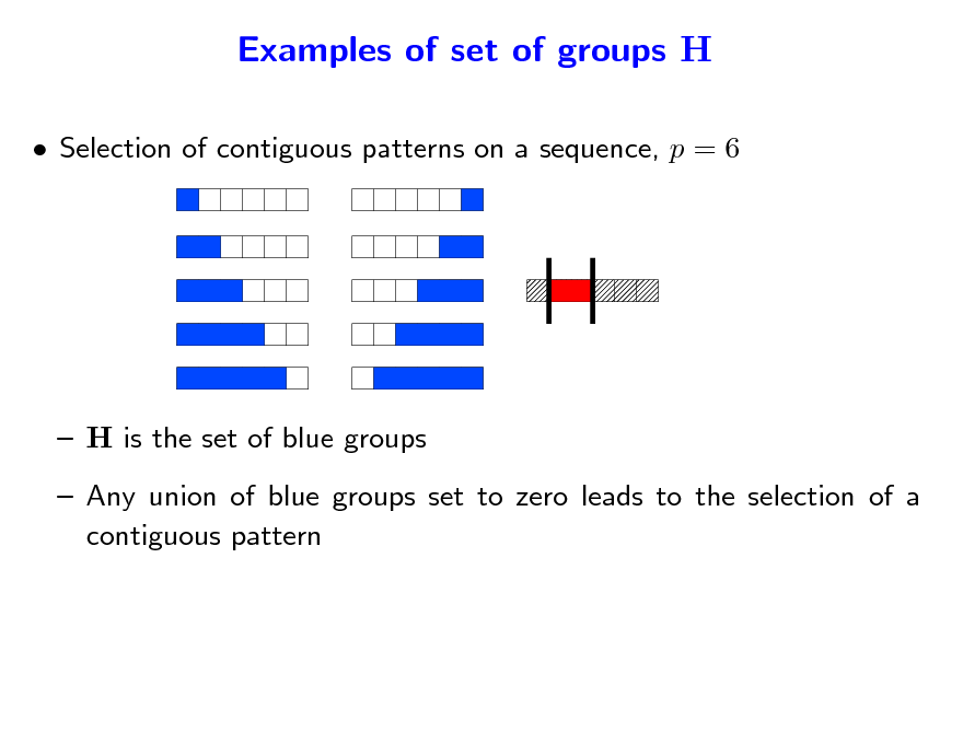
Examples of set of groups H
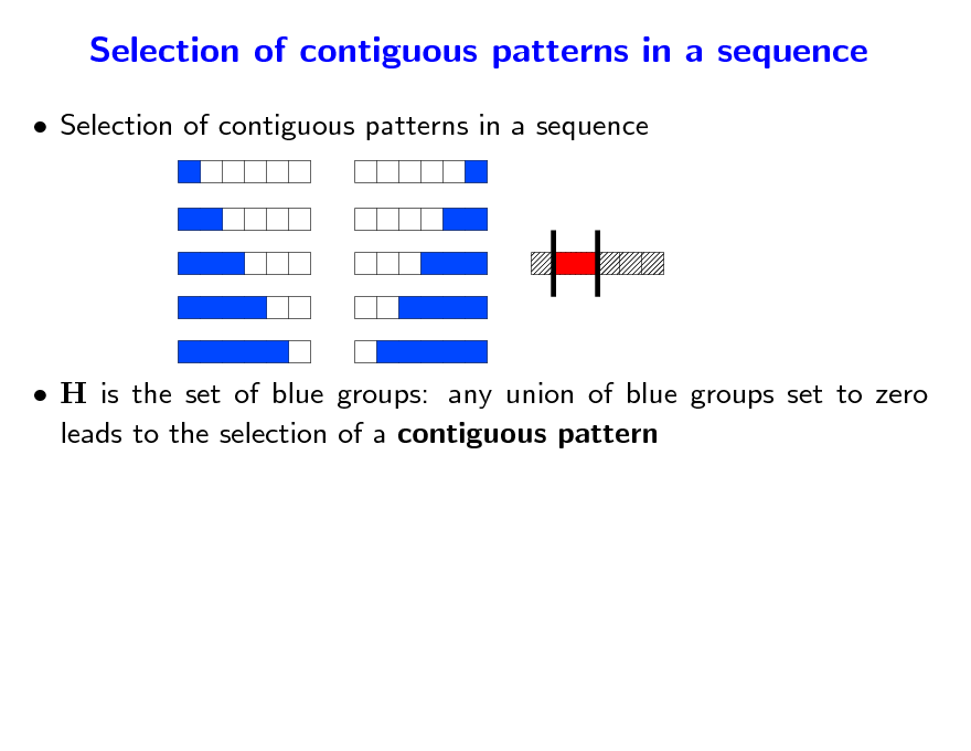
Selection of contiguous patterns on a sequence, p = 6
H is the set of blue groups Any union of blue groups set to zero leads to the selection of a contiguous pattern
117
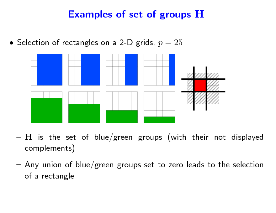
Examples of set of groups H
Selection of rectangles on a 2-D grids, p = 25
H is the set of blue/green groups (with their not displayed complements) Any union of blue/green groups set to zero leads to the selection of a rectangle
118
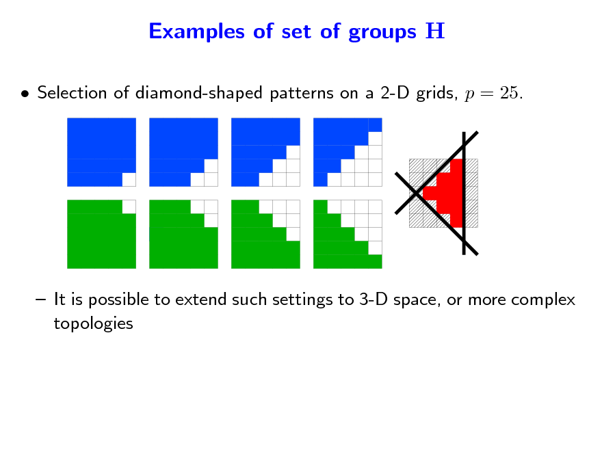
Examples of set of groups H
Selection of diamond-shaped patterns on a 2-D grids, p = 25.
It is possible to extend such settings to 3-D space, or more complex topologies
119
Unit norm balls Geometric interpretation
w
1
2 2 w1 + w2 + |w3|
w
2
+ |w1| + |w2|
120
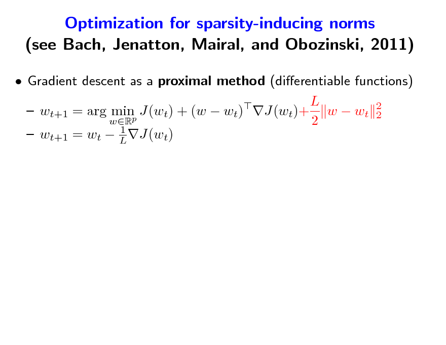
Optimization for sparsity-inducing norms (see Bach, Jenatton, Mairal, and Obozinski, 2011)
Gradient descent as a proximal method (dierentiable functions) L wt+1 = arg minp J(wt) + (w wt) J(wt)+ w wt 2 2 wR 2 1 wt+1 = wt L J(wt)
121
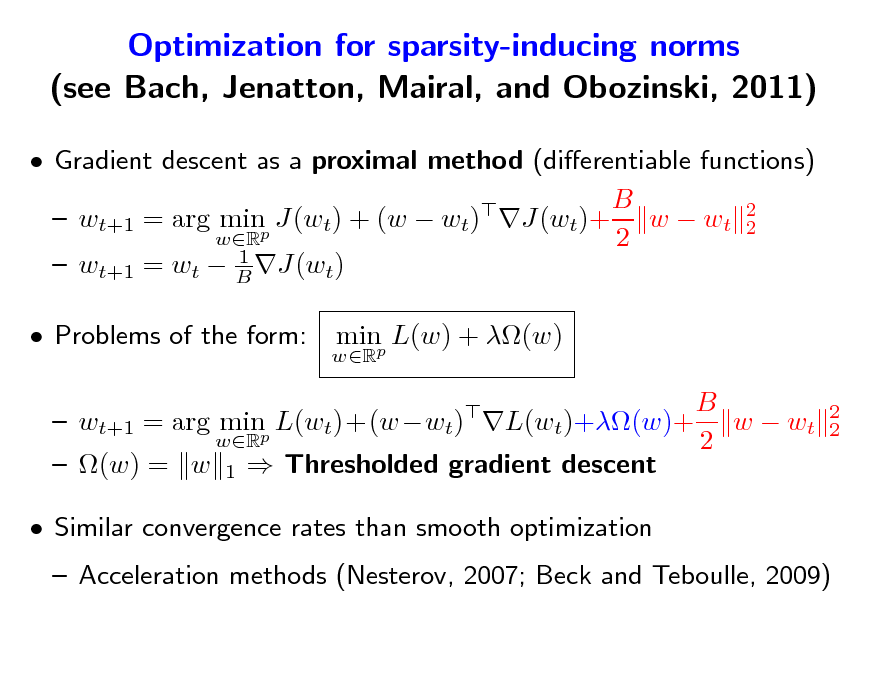
Optimization for sparsity-inducing norms (see Bach, Jenatton, Mairal, and Obozinski, 2011)
Gradient descent as a proximal method (dierentiable functions) B wt+1 = arg minp J(wt) + (w wt) J(wt)+ w wt 2 2 wR 2 1 wt+1 = wt B J(wt) Problems of the form:
wR
minp L(w) + (w)
2 2
B wt+1 = arg minp L(wt)+(wwt) L(wt)+(w)+ w wt wR 2 (w) = w 1 Thresholded gradient descent Similar convergence rates than smooth optimization
Acceleration methods (Nesterov, 2007; Beck and Teboulle, 2009)
122
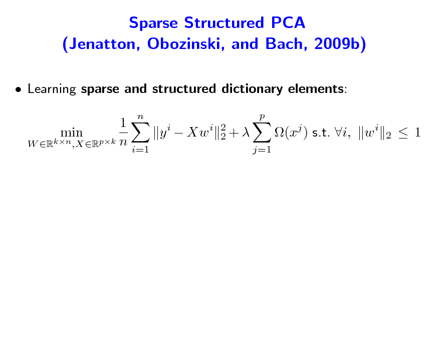
Sparse Structured PCA (Jenatton, Obozinski, and Bach, 2009b)
Learning sparse and structured dictionary elements: 1 y i Xw i min W Rkn ,XRpk n i=1
n p 2 2+ j=1
(xj ) s.t. i, w i
2
1
123
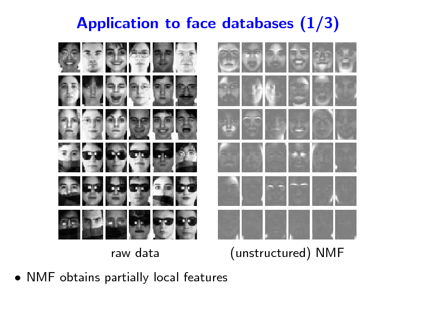
Application to face databases (1/3)
raw data NMF obtains partially local features
(unstructured) NMF
124
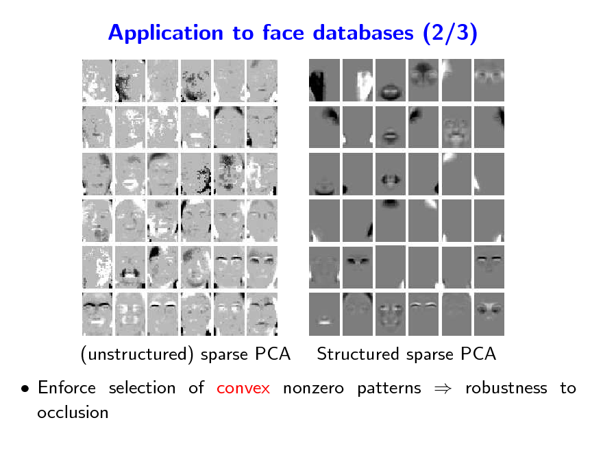
Application to face databases (2/3)
(unstructured) sparse PCA
Structured sparse PCA
Enforce selection of convex nonzero patterns robustness to occlusion
125
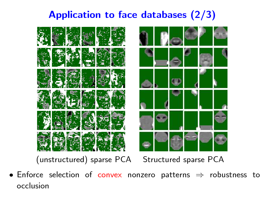
Application to face databases (2/3)
(unstructured) sparse PCA
Structured sparse PCA
Enforce selection of convex nonzero patterns robustness to occlusion
126
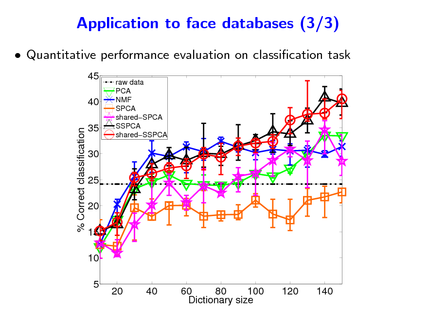
Application to face databases (3/3)
Quantitative performance evaluation on classication task
45 40 % Correct classification 35 30 25 20 15 10 5 20 40 60 80 100 Dictionary size 120 140
raw data PCA NMF SPCA sharedSPCA SSPCA sharedSSPCA
127
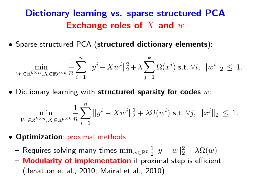
Dictionary learning vs. sparse structured PCA Exchange roles of X and w
Sparse structured PCA (structured dictionary elements): 1 y i Xw i min W Rkn ,XRpk n i=1
n k 2 2+ j=1
(xj ) s.t. i, w i
2
1.
Dictionary learning with structured sparsity for codes w: 1 min y i Xw i W Rkn ,XRpk n i=1 Optimization: proximal methods
n 2 2
+ (w i) s.t. j,
xj
2
1.
Requires solving many times minwRp 1 y w 2 + (w) 2 2 Modularity of implementation if proximal step is ecient (Jenatton et al., 2010; Mairal et al., 2010)
128
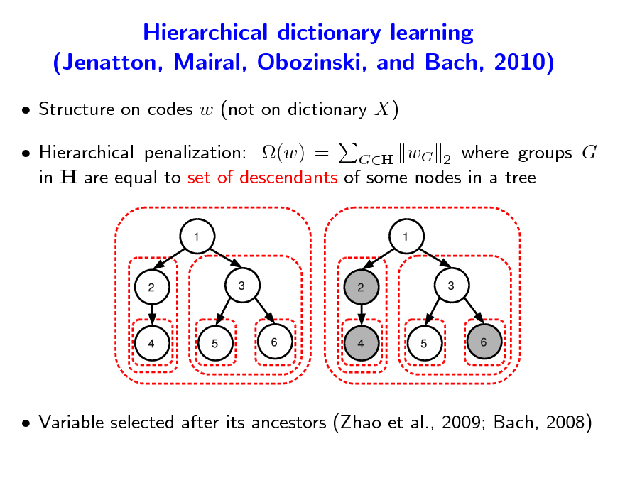
Hierarchical dictionary learning (Jenatton, Mairal, Obozinski, and Bach, 2010)
Structure on codes w (not on dictionary X) Hierarchical penalization: (w) = GH wG 2 where groups G in H are equal to set of descendants of some nodes in a tree
Variable selected after its ancestors (Zhao et al., 2009; Bach, 2008)
129
Hierarchical dictionary learning Modelling of text corpora
Each document is modelled through word counts Low-rank matrix factorization of word-document matrix Probabilistic topic models (Blei et al., 2003) Similar structures based on non parametric Bayesian methods (Blei et al., 2004) Can we achieve similar performance with simple matrix factorization formulation?
130
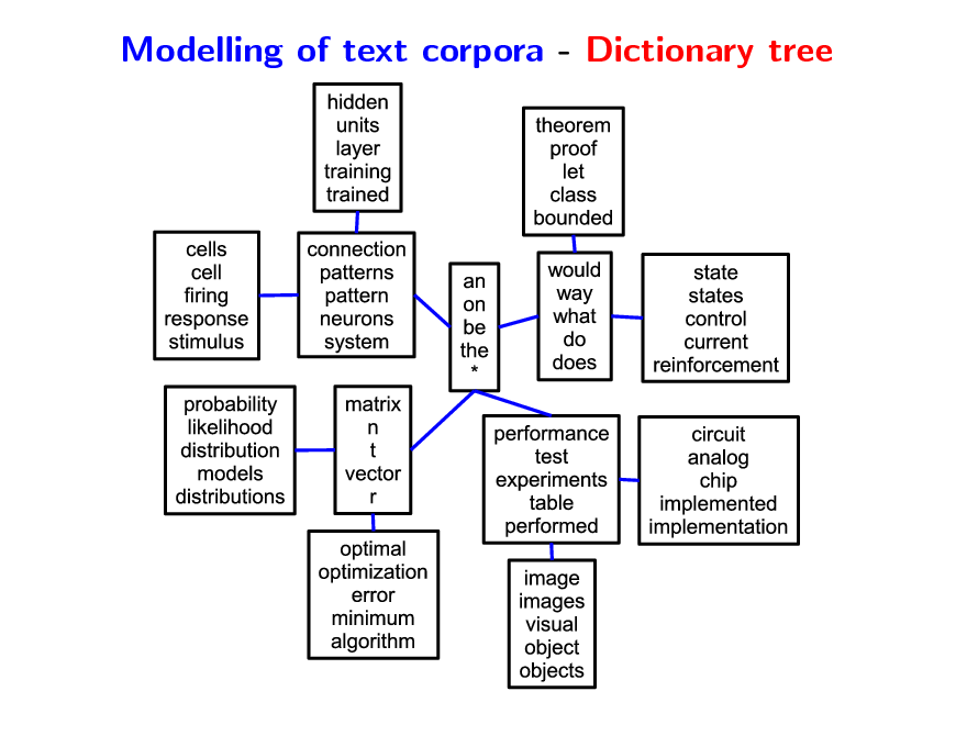
Modelling of text corpora - Dictionary tree
131
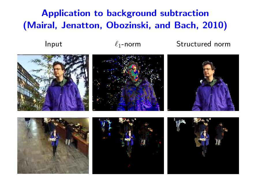
Application to background subtraction (Mairal, Jenatton, Obozinski, and Bach, 2010)
Input 1-norm Structured norm
132
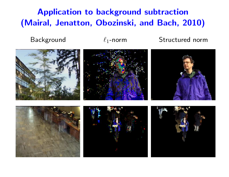
Application to background subtraction (Mairal, Jenatton, Obozinski, and Bach, 2010)
Background 1-norm Structured norm
133
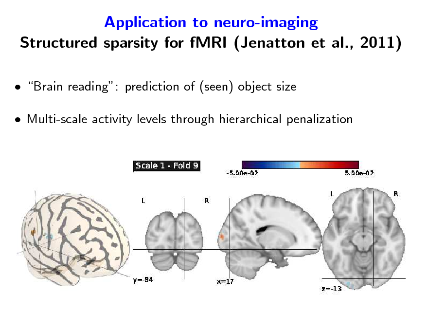
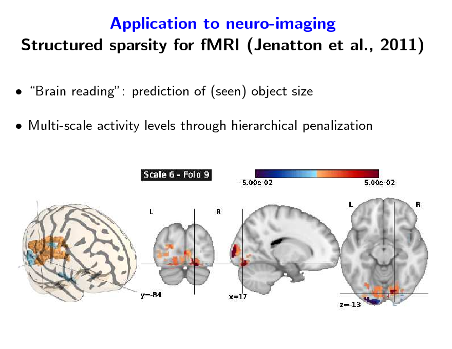
Application to neuro-imaging Structured sparsity for fMRI (Jenatton et al., 2011)
Brain reading: prediction of (seen) object size Multi-scale activity levels through hierarchical penalization
134
Application to neuro-imaging Structured sparsity for fMRI (Jenatton et al., 2011)
Brain reading: prediction of (seen) object size Multi-scale activity levels through hierarchical penalization
135
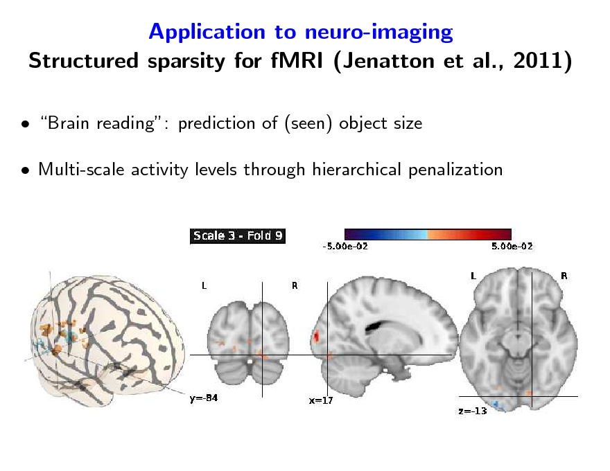
Application to neuro-imaging Structured sparsity for fMRI (Jenatton et al., 2011)
Brain reading: prediction of (seen) object size Multi-scale activity levels through hierarchical penalization
136
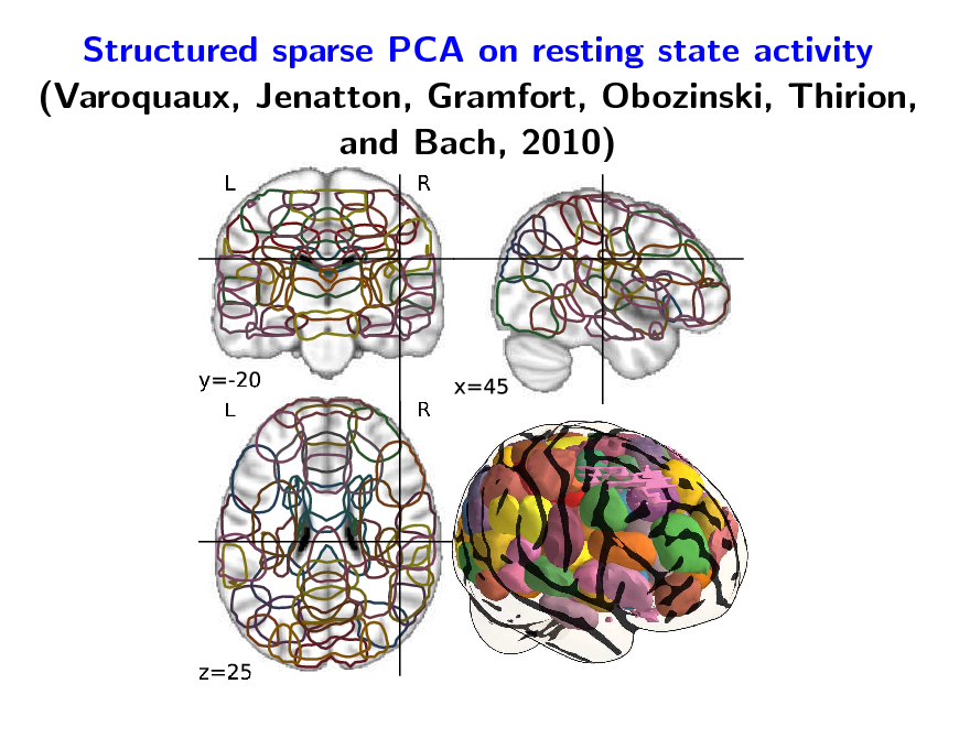
Structured sparse PCA on resting state activity (Varoquaux, Jenatton, Gramfort, Obozinski, Thirion, and Bach, 2010)
137
![Slide: 1-norm = convex envelope of cardinality of support
Let w Rp. Let V = {1, . . . , p} and Supp(w) = {j V, wj = 0} Cardinality of support: w
0
= Card(Supp(w))
Convex envelope = largest convex lower bound (see, e.g., Boyd and Vandenberghe, 2004)
||w|| 0
||w|| 1
1
1
1-norm = convex envelope of 0-quasi-norm on the -ball [1, 1]p](https://yosinski.com/mlss12/media/slides/MLSS-2012-Bach-Learning-with-Submodular-Functions_138.png)
1-norm = convex envelope of cardinality of support
Let w Rp. Let V = {1, . . . , p} and Supp(w) = {j V, wj = 0} Cardinality of support: w
0
= Card(Supp(w))
Convex envelope = largest convex lower bound (see, e.g., Boyd and Vandenberghe, 2004)
||w|| 0
||w|| 1
1
1
1-norm = convex envelope of 0-quasi-norm on the -ball [1, 1]p
138
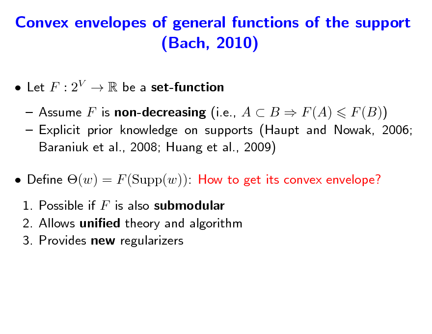
Convex envelopes of general functions of the support (Bach, 2010)
Let F : 2V R be a set-function Assume F is non-decreasing (i.e., A B F (A) F (B)) Explicit prior knowledge on supports (Haupt and Nowak, 2006; Baraniuk et al., 2008; Huang et al., 2009) Dene (w) = F (Supp(w)): How to get its convex envelope? 1. Possible if F is also submodular 2. Allows unied theory and algorithm 3. Provides new regularizers
139
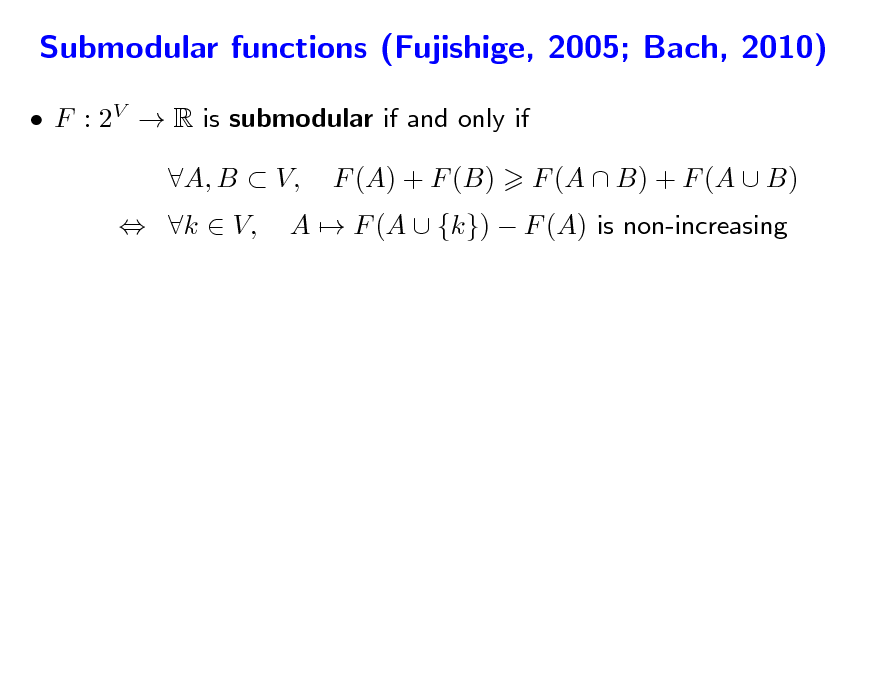
Submodular functions (Fujishige, 2005; Bach, 2010)
F : 2V R is submodular if and only if k V, A, B V, F (A) + F (B) A F (A {k}) F (A) is non-increasing F (A B) + F (A B)
140
Submodular functions (Fujishige, 2005; Bach, 2010)
F : 2V R is submodular if and only if k V, A, B V, F (A) + F (B) A F (A {k}) F (A) is non-increasing F (A B) + F (A B)
Intuition 1: dened like concave functions (diminishing returns) Example: F : A g(Card(A)) is submodular if g is concave
141
Submodular functions (Fujishige, 2005; Bach, 2010)
F : 2V R is submodular if and only if k V, A, B V, F (A) + F (B) A F (A {k}) F (A) is non-increasing F (A B) + F (A B)
Intuition 1: dened like concave functions (diminishing returns) Example: F : A g(Card(A)) is submodular if g is concave Polynomial-time minimization, conjugacy theory Intuition 2: behave like convex functions
142
Submodular functions (Fujishige, 2005; Bach, 2010)
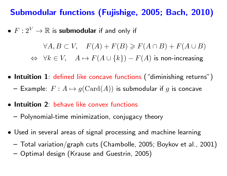
F : 2V R is submodular if and only if k V, A, B V, F (A) + F (B) A F (A {k}) F (A) is non-increasing F (A B) + F (A B)
Intuition 1: dened like concave functions (diminishing returns) Example: F : A g(Card(A)) is submodular if g is concave Polynomial-time minimization, conjugacy theory Intuition 2: behave like convex functions
Used in several areas of signal processing and machine learning
Total variation/graph cuts (Chambolle, 2005; Boykov et al., 2001) Optimal design (Krause and Guestrin, 2005)
143

Submodular functions - Examples
Concave functions of the cardinality: g(|A|) Cuts Entropies H((Xk )kA) from p random variables X1, . . . , Xp Gaussian variables H((Xk )kA) log det AA Functions of eigenvalues of sub-matrices Network ows Ecient representation for set covers Rank functions of matroids
144
![Slide: Submodular functions - Lovsz extension a
Subsets may be identied with elements of {0, 1}p Given any set-function F and w such that wj1
p
wjp , dene:
f (w) =
k=1
wjk [F ({j1, . . . , jk }) F ({j1, . . . , jk1})]
If w = 1A, f (w) = F (A) extension from {0, 1}p to Rp f is piecewise ane and positively homogeneous F is submodular if and only if f is convex (Lovsz, 1982) a](https://yosinski.com/mlss12/media/slides/MLSS-2012-Bach-Learning-with-Submodular-Functions_145.png)
Submodular functions - Lovsz extension a
Subsets may be identied with elements of {0, 1}p Given any set-function F and w such that wj1
p
wjp , dene:
f (w) =
k=1
wjk [F ({j1, . . . , jk }) F ({j1, . . . , jk1})]
If w = 1A, f (w) = F (A) extension from {0, 1}p to Rp f is piecewise ane and positively homogeneous F is submodular if and only if f is convex (Lovsz, 1982) a
145
Submodular functions and structured sparsity
Let F : 2V R be a non-decreasing submodular set-function Proposition: the convex envelope of : w F (Supp(w)) on the -ball is : w f (|w|) where f is the Lovsz extension of F a
146
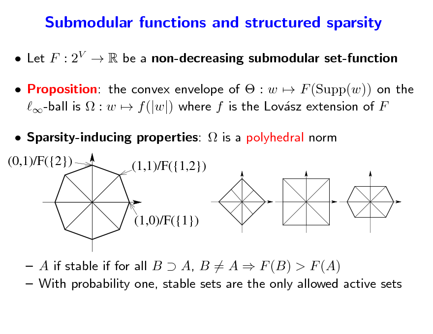
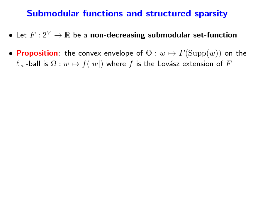
Submodular functions and structured sparsity
Let F : 2V R be a non-decreasing submodular set-function Proposition: the convex envelope of : w F (Supp(w)) on the -ball is : w f (|w|) where f is the Lovsz extension of F a Sparsity-inducing properties: is a polyhedral norm
(0,1)/F({2}) (1,1)/F({1,2})
(1,0)/F({1})
A if stable if for all B A, B = A F (B) > F (A) With probability one, stable sets are the only allowed active sets
147
Polyhedral unit balls
w3
w w
1
2
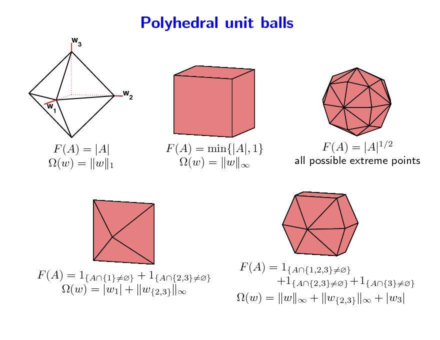
F (A) = |A| (w) = w 1
F (A) = min{|A|, 1} (w) = w
F (A) = |A|1/2 all possible extreme points
F (A) = 1{A{1}=} + 1{A{2,3}=} (w) = |w1| + w{2,3}
F (A) = 1{A{1,2,3}=} +1{A{2,3}=} +1{A{3}=} (w) = w + w{2,3} + |w3|
148
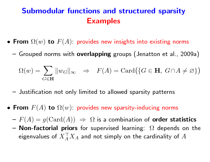
Submodular functions and structured sparsity Examples
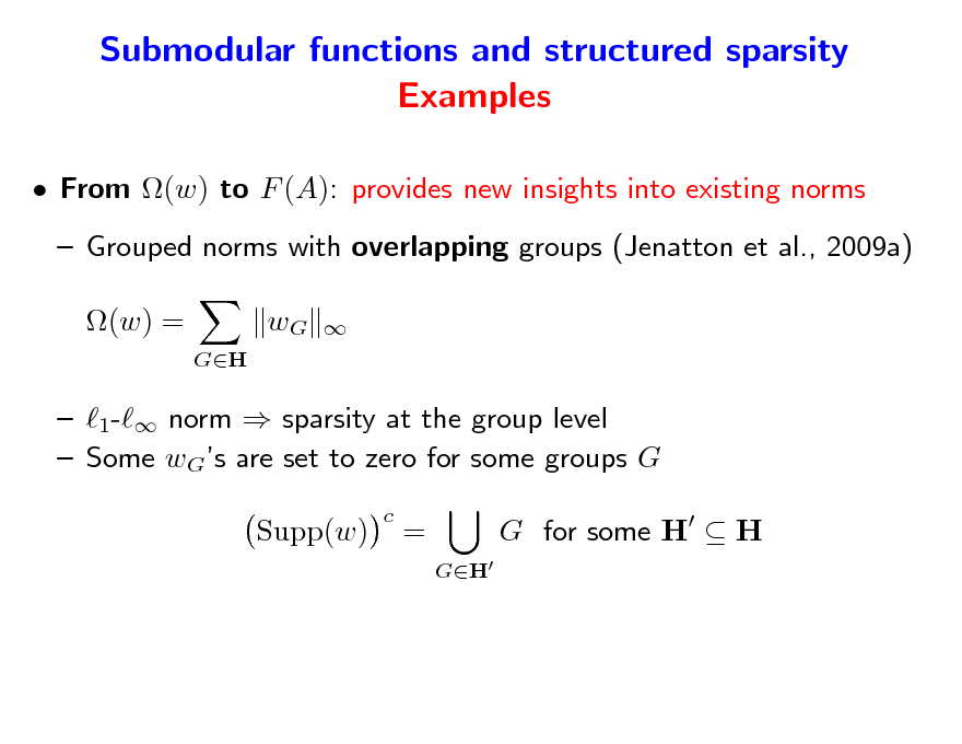
From (w) to F (A): provides new insights into existing norms Grouped norms with overlapping groups (Jenatton et al., 2009a) (w) =
GH
wG
1- norm sparsity at the group level Some wGs are set to zero for some groups G Supp(w)
c
=
GH
G for some H H
149
Submodular functions and structured sparsity Examples
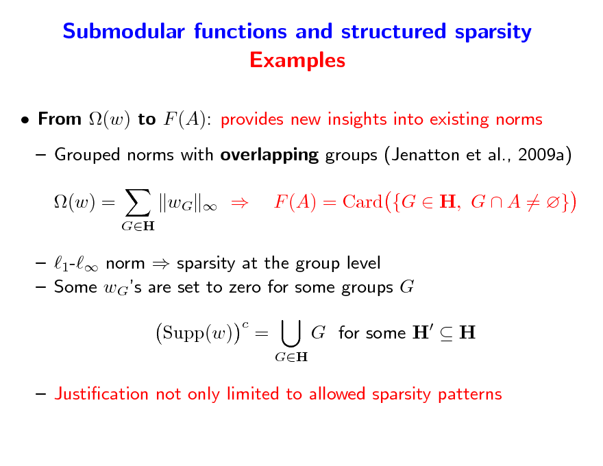
From (w) to F (A): provides new insights into existing norms Grouped norms with overlapping groups (Jenatton et al., 2009a) (w) =
GH
wG
F (A) = Card {G H, G A = }
1- norm sparsity at the group level Some wGs are set to zero for some groups G Supp(w)
c
=
GH
G for some H H
Justication not only limited to allowed sparsity patterns
150
Selection of contiguous patterns in a sequence
Selection of contiguous patterns in a sequence
H is the set of blue groups: any union of blue groups set to zero leads to the selection of a contiguous pattern
151
Selection of contiguous patterns in a sequence
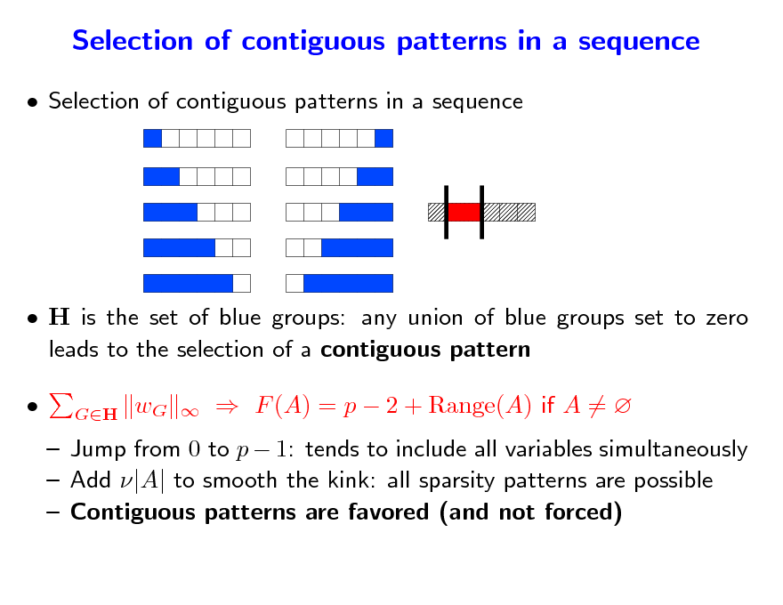
Selection of contiguous patterns in a sequence
H is the set of blue groups: any union of blue groups set to zero leads to the selection of a contiguous pattern
GH
wG
F (A) = p 2 + Range(A) if A =
Jump from 0 to p 1: tends to include all variables simultaneously Add |A| to smooth the kink: all sparsity patterns are possible Contiguous patterns are favored (and not forced)
152
Extensions of norms with overlapping groups
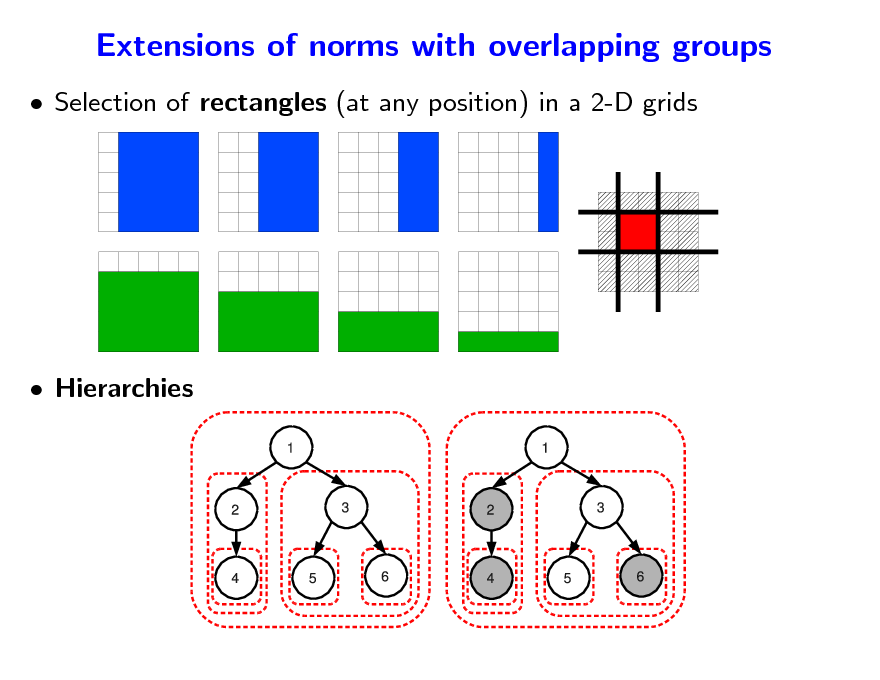
Selection of rectangles (at any position) in a 2-D grids
Hierarchies
153
Submodular functions and structured sparsity Examples
From (w) to F (A): provides new insights into existing norms Grouped norms with overlapping groups (Jenatton et al., 2009a) (w) =
GH
wG
F (A) = Card {G H, GA = }
Justication not only limited to allowed sparsity patterns
154
Submodular functions and structured sparsity Examples
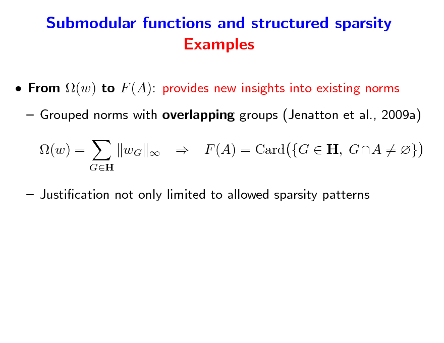
From (w) to F (A): provides new insights into existing norms Grouped norms with overlapping groups (Jenatton et al., 2009a) (w) =
GH
wG
F (A) = Card {G H, GA = }
Justication not only limited to allowed sparsity patterns From F (A) to (w): provides new sparsity-inducing norms F (A) = g(Card(A)) is a combination of order statistics Non-factorial priors for supervised learning: depends on the eigenvalues of XA XA and not simply on the cardinality of A
155
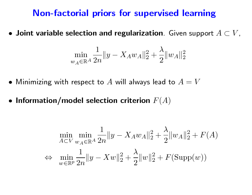
Non-factorial priors for supervised learning
Joint variable selection and regularization. Given support A V , 1 min y XAwA wA RA 2n
2 2
+ wA 2
2 2
Minimizing with respect to A will always lead to A = V Information/model selection criterion F (A) 1 2 min min y XAwA 2 + wA 2 + F (A) 2 AV wA RA 2n 2 1 2 y Xw 2 + w 2 + F (Supp(w)) minp 2 wR 2n 2
156
Non-factorial priors for supervised learning
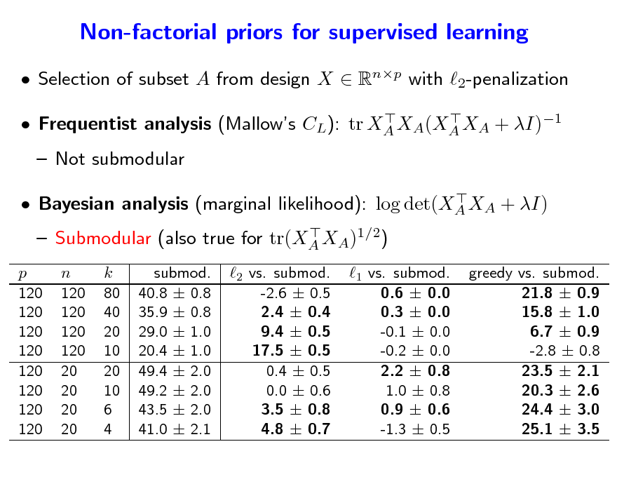
Selection of subset A from design X Rnp with 2-penalization
Frequentist analysis (Mallows CL): tr XA XA(XA XA + I)1
Not submodular
Bayesian analysis (marginal likelihood): log det(XA XA + I) Submodular (also true for tr(XA XA)1/2)
p 120 120 120 120 120 120 120 120
n 120 120 120 120 20 20 20 20
k 80 40 20 10 20 10 6 4
submod. 40.8 0.8 35.9 0.8 29.0 1.0 20.4 1.0 49.4 2.0 49.2 2.0 43.5 2.0 41.0 2.1
2 vs. submod. -2.6 0.5 2.4 0.4 9.4 0.5 17.5 0.5 0.4 0.5 0.0 0.6 3.5 0.8 4.8 0.7
1 vs. submod. 0.6 0.0 0.3 0.0 -0.1 0.0 -0.2 0.0 2.2 0.8 1.0 0.8 0.9 0.6 -1.3 0.5
greedy vs. submod. 21.8 0.9 15.8 1.0 6.7 0.9 -2.8 0.8 23.5 2.1 20.3 2.6 24.4 3.0 25.1 3.5
157
Unied optimization algorithms
Polyhedral norm with O(3p) faces and extreme points Not suitable to linear programming toolboxes Subgradient (w (w) non-dierentiable)
subgradient may be obtained in polynomial time too slow
158
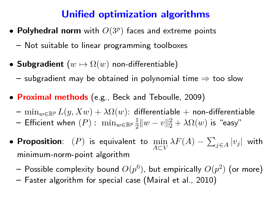
Unied optimization algorithms
Polyhedral norm with O(3p) faces and extreme points Not suitable to linear programming toolboxes Subgradient (w (w) non-dierentiable)
subgradient may be obtained in polynomial time too slow minwRp L(y, Xw) + (w): dierentiable + non-dierentiable 1 Ecient when (P ) : minwRp 2 w v 2 + (w) is easy 2 minimum-norm-point algorithm
AV jA |vj |
Proximal methods (e.g., Beck and Teboulle, 2009)
Proposition: (P ) is equivalent to min F (A)
with
Possible complexity bound O(p6), but empirically O(p2) (or more) Faster algorithm for special case (Mairal et al., 2010)
159
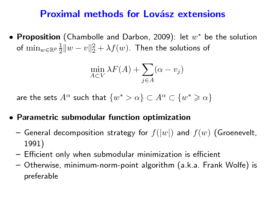
Proximal methods for Lovsz extensions a
Proposition (Chambolle and Darbon, 2009): let w be the solution 1 of minwRp 2 w v 2 + f (w). Then the solutions of 2
AV
min F (A) +
jA
( vj ) }
are the sets A such that {w > } A {w Parametric submodular function optimization
General decomposition strategy for f (|w|) and f (w) (Groenevelt, 1991) Ecient only when submodular minimization is ecient Otherwise, minimum-norm-point algorithm (a.k.a. Frank Wolfe) is preferable
160
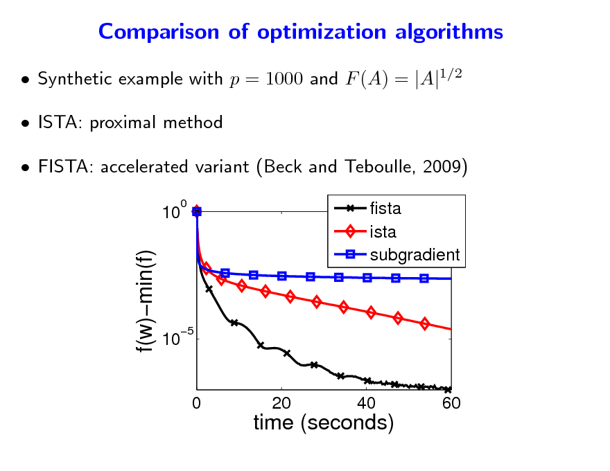
Comparison of optimization algorithms
Synthetic example with p = 1000 and F (A) = |A|1/2 ISTA: proximal method FISTA: accelerated variant (Beck and Teboulle, 2009)
10
0
f(w)min(f)
fista ista subgradient
10
5
0
20
40
60
time (seconds)
161
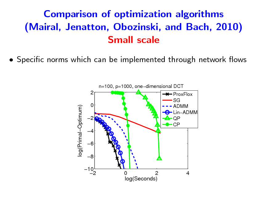
Comparison of optimization algorithms (Mairal, Jenatton, Obozinski, and Bach, 2010) Small scale
Specic norms which can be implemented through network ows
n=100, p=1000, onedimensional DCT
2 log(PrimalOptimum) 0 2 4 6 8 10 2 0 2 log(Seconds)
ProxFlox SG ADMM LinADMM QP CP
4
162
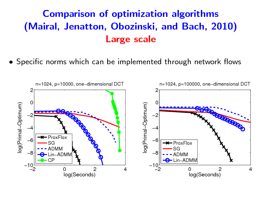
Comparison of optimization algorithms (Mairal, Jenatton, Obozinski, and Bach, 2010) Large scale
Specic norms which can be implemented through network ows
n=1024, p=10000, onedimensional DCT n=1024, p=100000, onedimensional DCT
2 log(PrimalOptimum) log(PrimalOptimum) 0 2 4 6 8 10 2
ProxFlox SG ADMM LinADMM CP
2 0 2 4 6 8 10 2
ProxFlox SG ADMM LinADMM
0 2 log(Seconds)
4
0 2 log(Seconds)
4
163
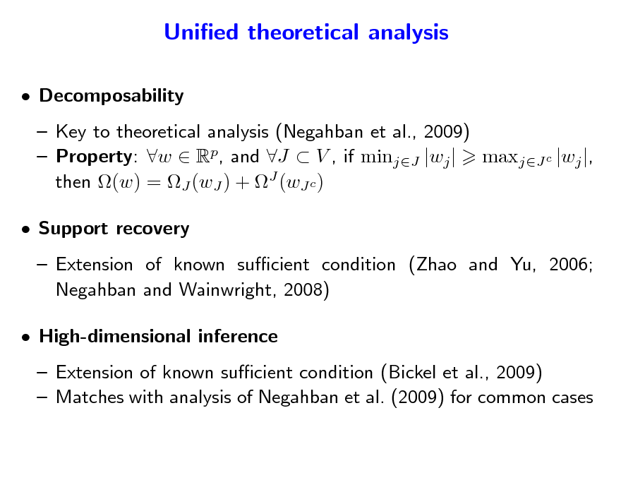
Unied theoretical analysis
Decomposability Key to theoretical analysis (Negahban et al., 2009) Property: w Rp, and J V , if minjJ |wj | maxjJ c |wj |, then (w) = J (wJ ) + J (wJ c ) Support recovery Extension of known sucient condition (Zhao and Yu, 2006; Negahban and Wainwright, 2008) High-dimensional inference Extension of known sucient condition (Bickel et al., 2009) Matches with analysis of Negahban et al. (2009) for common cases
164
![Slide: Support recovery - minwRp
Notation
1 2n
y Xw
2 2
+ (w)
(J) = minBJ c F (BJ)F (J) (0, 1] (for J stable) F (B) c(J) = supwRp J (wJ )/ wJ 2 |J|1/2 maxkV F ({k}) Assume y = Xw + , with N (0, I) J = smallest stable set containing the support of w Assume = minj,wj =0 |wj | > 0 1 Let Q = n X X Rpp. Assume = min(QJJ ) > 0
(J) n 2
Proposition
Assume that for > 0, (J )[(J (Q1QJj ))jJ c ] 1 JJ If 2c(J) , w has support equal to J, with probability larger than 1 3P (z) > z is a multivariate normal with covariance matrix Q](https://yosinski.com/mlss12/media/slides/MLSS-2012-Bach-Learning-with-Submodular-Functions_165.png)
Support recovery - minwRp
Notation
1 2n
y Xw
2 2
+ (w)
(J) = minBJ c F (BJ)F (J) (0, 1] (for J stable) F (B) c(J) = supwRp J (wJ )/ wJ 2 |J|1/2 maxkV F ({k}) Assume y = Xw + , with N (0, I) J = smallest stable set containing the support of w Assume = minj,wj =0 |wj | > 0 1 Let Q = n X X Rpp. Assume = min(QJJ ) > 0
(J) n 2
Proposition
Assume that for > 0, (J )[(J (Q1QJj ))jJ c ] 1 JJ If 2c(J) , w has support equal to J, with probability larger than 1 3P (z) > z is a multivariate normal with covariance matrix Q
165
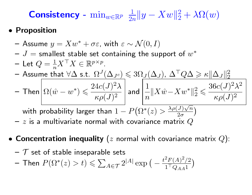
Consistency - minwRp
Proposition
1 2n
y Xw
2 2
+ (w)
Assume y = Xw + , with N (0, I) J = smallest stable set containing the support of w 1 Let Q = n X X Rpp. Assume that s.t. J (J c ) 3J (J ), Q J 24c(J)2 1 and X wXw 2 (J) n
2 2 (J) n 2
2 2
Then (w w )
36c(J)22 (J)2
with probability larger than 1 P (z) > z is a multivariate normal with covariance matrix Q Concentration inequality (z normal with covariance matrix Q): T set of stable inseparable sets t2 F (A)2 /2 |A| exp 1Q 1 Then P ( (z) > t) AT 2
AA
166
![Slide: Symmetric submodular functions (Bach, 2011)
Let F : 2V R be a symmetric submodular set-function Proposition: The Lovsz extension f (w) is the convex envelope of a the function w maxR F ({w }) on the set [0, 1]p + R1V = {w Rp, maxkV wk minkV wk 1}.](https://yosinski.com/mlss12/media/slides/MLSS-2012-Bach-Learning-with-Submodular-Functions_167.png)
Symmetric submodular functions (Bach, 2011)
Let F : 2V R be a symmetric submodular set-function Proposition: The Lovsz extension f (w) is the convex envelope of a the function w maxR F ({w }) on the set [0, 1]p + R1V = {w Rp, maxkV wk minkV wk 1}.
167
![Slide: Symmetric submodular functions (Bach, 2011)
Let F : 2V R be a symmetric submodular set-function Proposition: The Lovsz extension f (w) is the convex envelope of a the function w maxR F ({w }) on the set [0, 1]p + R1V = {w Rp, maxkV wk minkV wk 1}.
w1=w2 w3> w1>w2 (1,0,1)/F({1,3}) w1> w3>w2 (1,0,0)/F({1}) w2=w3 w1> w2>w3 (0,0,1)/F({3}) w3> w2>w1 (0,1,1)/F({2,3}) w2> w3>w1 (0,1,0)/F({2}) w2> w1>w3 w1=w3 (1,1,0)/F({1,2})
(1,0,1)/2 (1,0,0) (1,1,0) (0,0,1) (0,1,1) (0,1,0)/2](https://yosinski.com/mlss12/media/slides/MLSS-2012-Bach-Learning-with-Submodular-Functions_168.png)
Symmetric submodular functions (Bach, 2011)
Let F : 2V R be a symmetric submodular set-function Proposition: The Lovsz extension f (w) is the convex envelope of a the function w maxR F ({w }) on the set [0, 1]p + R1V = {w Rp, maxkV wk minkV wk 1}.
w1=w2 w3> w1>w2 (1,0,1)/F({1,3}) w1> w3>w2 (1,0,0)/F({1}) w2=w3 w1> w2>w3 (0,0,1)/F({3}) w3> w2>w1 (0,1,1)/F({2,3}) w2> w3>w1 (0,1,0)/F({2}) w2> w1>w3 w1=w3 (1,1,0)/F({1,2})
(1,0,1)/2 (1,0,0) (1,1,0) (0,0,1) (0,1,1) (0,1,0)/2
168
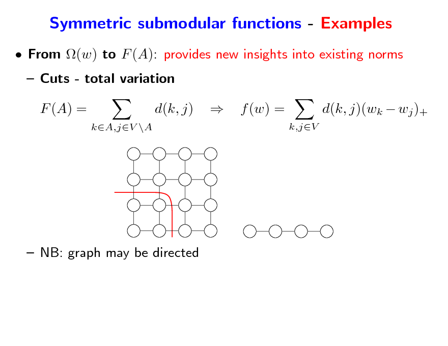
Symmetric submodular functions - Examples
From (w) to F (A): provides new insights into existing norms Cuts - total variation F (A) =
kA,jV \A
d(k, j)
f (w) =
k,jV
d(k, j)(wk wj )+
NB: graph may be directed
169
Symmetric submodular functions - Examples
From F (A) to (w): provides new sparsity-inducing norms
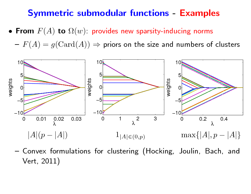
10 5 weights weights 0 5 10 0 10 5 0 5 10 0 weights 1 2 3 10 5 0 5 10 0
F (A) = g(Card(A)) priors on the size and numbers of clusters
0.01
0.02
0.03
0.2
0.4
|A|(p |A|)
1|A|(0,p)
max{|A|, p |A|}
Convex formulations for clustering (Hocking, Joulin, Bach, and Vert, 2011)
170
Symmetric submodular functions - Examples
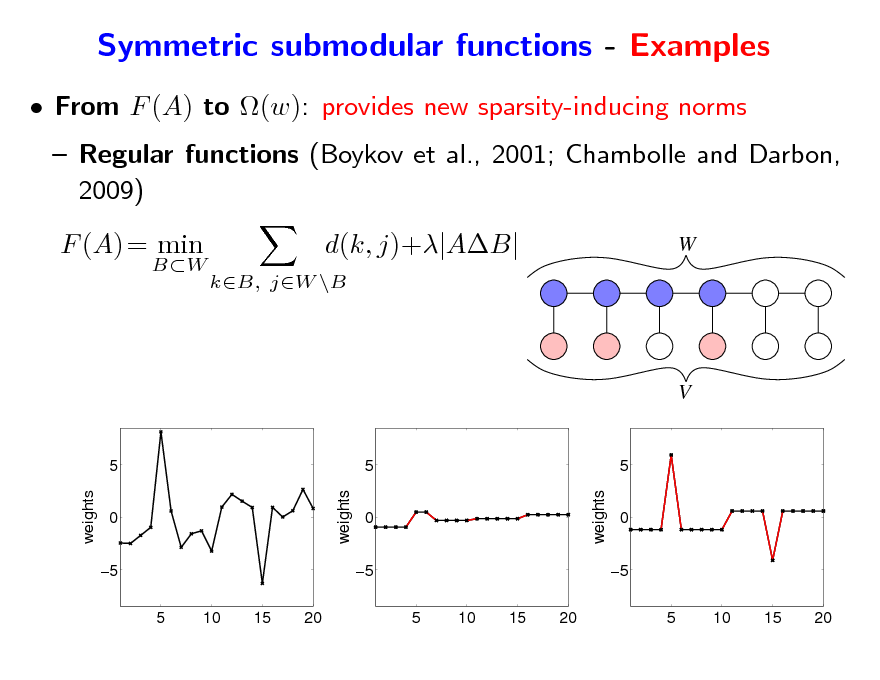
From F (A) to (w): provides new sparsity-inducing norms Regular functions (Boykov et al., 2001; Chambolle and Darbon, 2009) F (A) = min
BW
d(k, j)+|AB|
kB, jW \B
W
V
5 weights weights 0 5 5 10 15 20
5 0 5 5 10 15 20 weights
5 0 5 5 10 15 20
171
![Slide: q -relaxation of combinatorial penalties (Obozinski and Bach, 2011)
Main result of Bach (2010): Problems: f (|w|) is the convex envelope of F (Supp(w)) on [1, 1]p
Limited to submodular functions Limited to -relaxation: undesired artefacts
(1,1)/F({1,2})
(0,1)/F({2})
(1,0)/F({1})](https://yosinski.com/mlss12/media/slides/MLSS-2012-Bach-Learning-with-Submodular-Functions_172.png)
q -relaxation of combinatorial penalties (Obozinski and Bach, 2011)
Main result of Bach (2010): Problems: f (|w|) is the convex envelope of F (Supp(w)) on [1, 1]p
Limited to submodular functions Limited to -relaxation: undesired artefacts
(1,1)/F({1,2})
(0,1)/F({2})
(1,0)/F({1})
172

From to 2
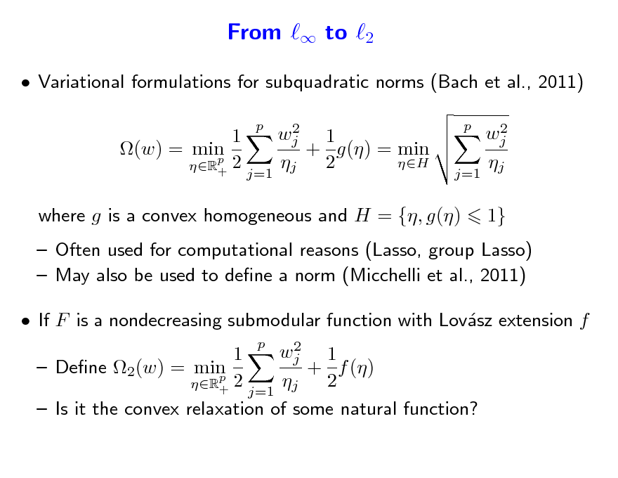
Variational formulations for subquadratic norms (Bach et al., 2011)
2 wj 1 1 (w) = min + g() = min p 2 H 2 R+ j=1 j p 2 wj j=1 j p
where g is a convex homogeneous and H = {, g()
1}
Often used for computational reasons (Lasso, group Lasso) May also be used to dene a norm (Micchelli et al., 2011)
173
From to 2
Variational formulations for subquadratic norms (Bach et al., 2011)
2 wj 1 1 + g() = min (w) = min p 2 H 2 R+ j=1 j p 2 wj j=1 j p
where g is a convex homogeneous and H = {, g()
1}
Often used for computational reasons (Lasso, group Lasso) May also be used to dene a norm (Micchelli et al., 2011) If F is a nondecreasing submodular function with Lovsz extension f a
2 wj 1 1 Dene 2(w) = min + f () p 2 2 R+ j=1 j Is it the convex relaxation of some natural function? p
174
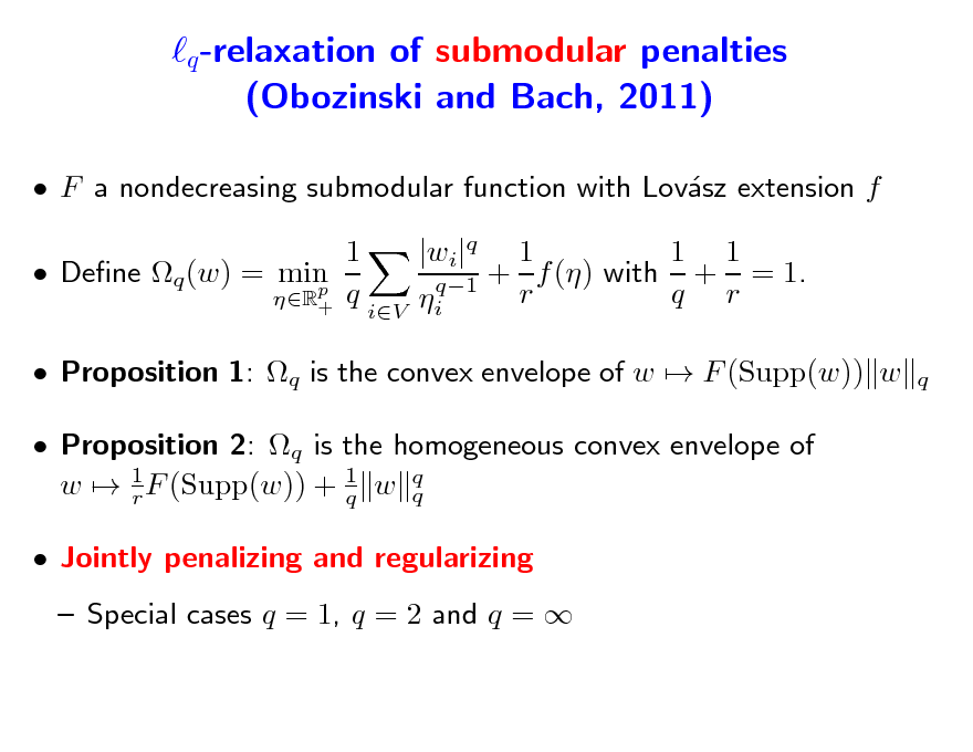
q -relaxation of submodular penalties (Obozinski and Bach, 2011)
F a nondecreasing submodular function with Lovsz extension f a 1 Dene q (w) = min p R+ q 1 1 |wi|q 1 q1 + r f () with q + r = 1. i
q
iV
Proposition 1: q is the convex envelope of w F (Supp(w)) w Proposition 2: q is the homogeneous convex envelope of w 1 F (Supp(w)) + 1 w q q r q Jointly penalizing and regularizing Special cases q = 1, q = 2 and q =
175
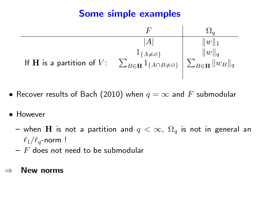
Some simple examples
F |A| q w 1 w q BH wB
If H is a partition of V :
1{A=} BH 1{AB=}
q
Recover results of Bach (2010) when q = and F submodular However when H is not a partition and q < , q is not in general an 1/q -norm ! F does not need to be submodular New norms
176
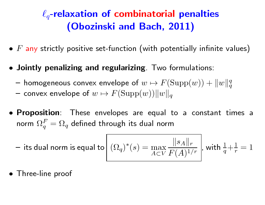
q -relaxation of combinatorial penalties (Obozinski and Bach, 2011)
F any strictly positive set-function (with potentially innite values) Jointly penalizing and regularizing. Two formulations: homogeneous convex envelope of w F (Supp(w)) + w convex envelope of w F (Supp(w)) w q
q q
Proposition: These envelopes are equal to a constant times a norm F = q dened through its dual norm q sA r its dual norm is equal to (q ) (s) = max , with 1 + 1 = 1 q r AV F (A)1/r
Three-line proof
177
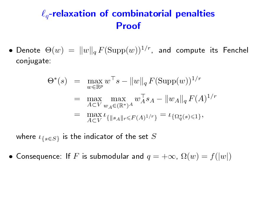
q -relaxation of combinatorial penalties Proof
Denote (w) = conjugate: w F (Supp(w))1/r , and compute its Fenchel q
(s) = max w s w p
wR
F (Supp(w))1/r q
q
= max
AV
= max {
AV wA (R )A
max
wA sA wA
F (A)1/r
1} ,
sA r F (A)1/r }
= {(s) q
where {sS} is the indicator of the set S Consequence: If F is submodular and q = +, (w) = f (|w|)
178
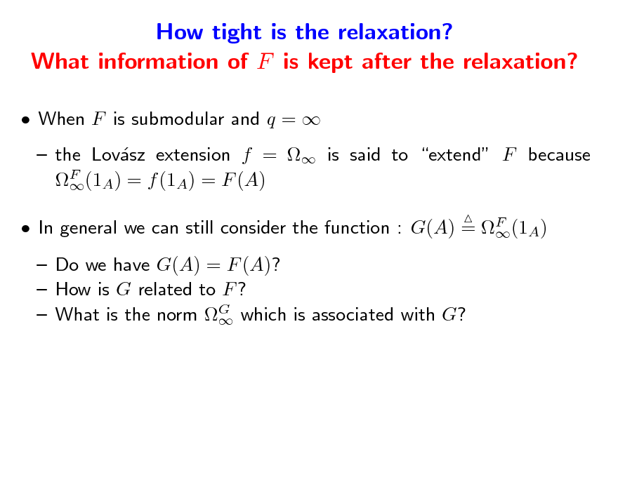
How tight is the relaxation? What information of F is kept after the relaxation?
When F is submodular and q = the Lovsz extension f = is said to extend F because a F (1A) = f (1A) = F (A) In general we can still consider the function : G(A) = F (1A) Do we have G(A) = F (A)? How is G related to F ? What is the norm G which is associated with G?
179
Lower combinatorial envelope
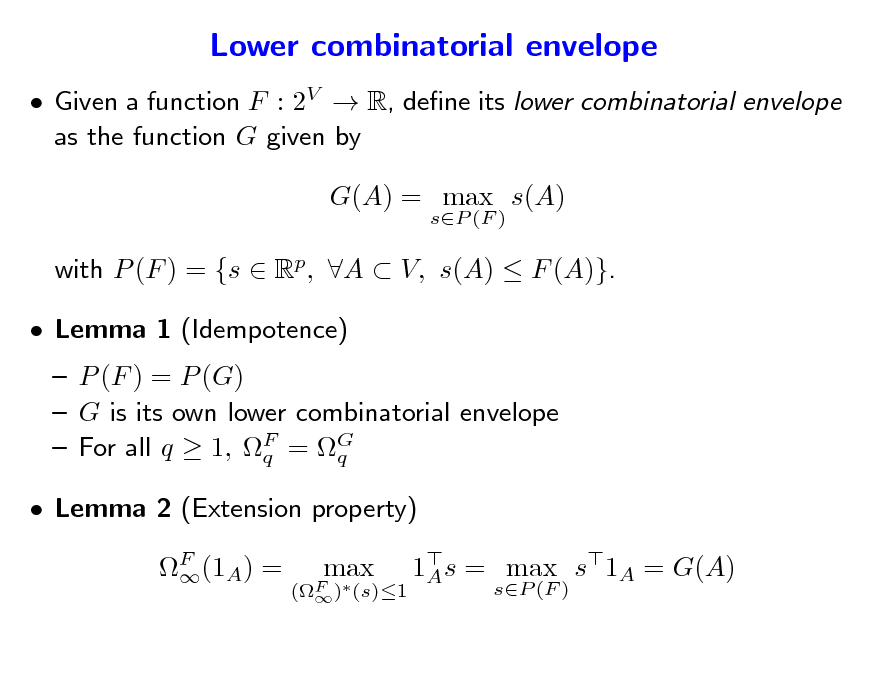
Given a function F : 2V R, dene its lower combinatorial envelope as the function G given by G(A) = max s(A)
sP (F )
with P (F ) = {s Rp, A V, s(A) F (A)}. Lemma 1 (Idempotence) P (F ) = P (G) G is its own lower combinatorial envelope For all q 1, F = G q q F (1A) = 1s = max s1A = G(A) A
sP (F )
Lemma 2 (Extension property)
(F ) (s)1
max
180
Conclusion
Structured sparsity for machine learning and statistics Many applications (image, audio, text, etc.) May be achieved through structured sparsity-inducing norms Link with submodular functions: unied analysis and algorithms
181
Conclusion
Structured sparsity for machine learning and statistics Many applications (image, audio, text, etc.) May be achieved through structured sparsity-inducing norms Link with submodular functions: unied analysis and algorithms On-going work on structured sparsity Norm design beyond submodular functions Instance of general framework of Chandrasekaran et al. (2010) Links with greedy methods (Haupt and Nowak, 2006; Baraniuk et al., 2008; Huang et al., 2009) Links between norm , support Supp(w), and design X (see, e.g., Grave, Obozinski, and Bach, 2011) Achieving log p = O(n) algorithmically (Bach, 2008)
182
Conclusion
Submodular functions to encode discrete structures Structured sparsity-inducing norms Convex optimization for submodular function optimization Approximate optimization using classical iterative algorithms Future work Primal-dual optimization Going beyond linear programming
183
References
F. Bach. Exploring large feature spaces with hierarchical multiple kernel learning. In Advances in Neural Information Processing Systems, 2008. F. Bach. Structured sparsity-inducing norms through submodular functions. In NIPS, 2010. F. Bach. Convex analysis and optimization with submodular functions: a tutorial. Technical Report 00527714, HAL, 2010. F. Bach. Learning with Submodular Functions: A Convex Optimization Perspective. 2011. URL http://hal.inria.fr/hal-00645271/en. F. Bach. Shaping level sets with submodular functions. In Adv. NIPS, 2011. F. Bach, R. Jenatton, J. Mairal, and G. Obozinski. Optimization with sparsity-inducing penalties. Technical Report 00613125, HAL, 2011. R. G. Baraniuk, V. Cevher, M. F. Duarte, and C. Hegde. Model-based compressive sensing. Technical report, arXiv:0808.3572, 2008. A. Beck and M. Teboulle. A fast iterative shrinkage-thresholding algorithm for linear inverse problems. SIAM Journal on Imaging Sciences, 2(1):183202, 2009. M. J. Best and N. Chakravarti. Active set algorithms for isotonic regression; a unifying framework. Mathematical Programming, 47(1):425439, 1990. P. Bickel, Y. Ritov, and A. Tsybakov. Simultaneous analysis of Lasso and Dantzig selector. Annals of Statistics, 37(4):17051732, 2009.
184
D. Blei, A. Ng, and M. Jordan. Latent dirichlet allocation. The Journal of Machine Learning Research, 3:9931022, January 2003. D. Blei, T.L. Griths, M.I. Jordan, and J.B. Tenenbaum. Hierarchical topic models and the nested Chinese restaurant process. Advances in neural information processing systems, 16:106, 2004. L. Bottou and O. Bousquet. The tradeos of large scale learning. In Advances in Neural Information Processing Systems (NIPS), volume 20, 2008. S. P. Boyd and L. Vandenberghe. Convex Optimization. Cambridge University Press, 2004. Y. Boykov, O. Veksler, and R. Zabih. Fast approximate energy minimization via graph cuts. IEEE Trans. PAMI, 23(11):12221239, 2001. V. Cevher, M. F. Duarte, C. Hegde, and R. G. Baraniuk. Sparse signal recovery using markov random elds. In Advances in Neural Information Processing Systems, 2008. A. Chambolle. Total variation minimization and a class of binary MRF models. In Energy Minimization Methods in Computer Vision and Pattern Recognition, pages 136152. Springer, 2005. A. Chambolle and J. Darbon. On total variation minimization and surface evolution using parametric maximum ows. International Journal of Computer Vision, 84(3):288307, 2009. V. Chandrasekaran, B. Recht, P.A. Parrilo, and A.S. Willsky. The convex geometry of linear inverse problems. Arxiv preprint arXiv:1012.0621, 2010. S. S. Chen, D. L. Donoho, and M. A. Saunders. Atomic decomposition by basis pursuit. SIAM Review, 43(1):129159, 2001. T. M. Cover and J. A. Thomas. Elements of Information Theory. John Wiley & Sons, 1991. J. Edmonds. Submodular functions, matroids, and certain polyhedra. In Combinatorial optimization -
185
Eureka, you shrink!, pages 1126. Springer, 1970. M. Elad and M. Aharon. Image denoising via sparse and redundant representations over learned dictionaries. IEEE Transactions on Image Processing, 15(12):37363745, 2006. U. Feige, V.S. Mirrokni, and J. Vondrak. Maximizing non-monotone submodular functions. In Proc. Symposium on Foundations of Computer Science, pages 461471. IEEE Computer Society, 2007. S. Fujishige. Submodular Functions and Optimization. Elsevier, 2005. S. Fujishige and S. Isotani. A submodular function minimization algorithm based on the minimum-norm base. Pacic Journal of Optimization, 7:317, 2011. A. Gramfort and M. Kowalski. Improving M/EEG source localization with an inter-condition sparse prior. In IEEE International Symposium on Biomedical Imaging, 2009. E. Grave, G. Obozinski, and F. Bach. Trace lasso: a trace norm regularization for correlated designs. Arxiv preprint arXiv:1109.1990, 2011. H. Groenevelt. Two algorithms for maximizing a separable concave function over a polymatroid feasible region. European Journal of Operational Research, 54(2):227236, 1991. J. Haupt and R. Nowak. Signal reconstruction from noisy random projections. IEEE Transactions on Information Theory, 52(9):40364048, 2006. T. Hocking, A. Joulin, F. Bach, and J.-P. Vert. Clusterpath: an algorithm for clustering using convex fusion penalties. In Proc. ICML, 2011. J. Huang, T. Zhang, and D. Metaxas. Learning with structured sparsity. In Proceedings of the 26th International Conference on Machine Learning (ICML), 2009. A. Hyvrinen, J. Karhunen, and E. Oja. Independent Component Analysis. John Wiley & Sons, 2001. a
186
S. Iwata, L. Fleischer, and S. Fujishige. A combinatorial strongly polynomial algorithm for minimizing submodular functions. Journal of the ACM, 48(4):761777, 2001. Stefanie Jegelka, Hui Lin, and Je A. Bilmes. Fast approximate submodular minimization. In Neural Information Processing Society (NIPS), Granada, Spain, December 2011. R. Jenatton, J.Y. Audibert, and F. Bach. Structured variable selection with sparsity-inducing norms. Technical report, arXiv:0904.3523, 2009a. R. Jenatton, G. Obozinski, and F. Bach. Structured sparse principal component analysis. Technical report, arXiv:0909.1440, 2009b. R. Jenatton, J. Mairal, G. Obozinski, and F. Bach. Proximal methods for sparse hierarchical dictionary learning. In Submitted to ICML, 2010. R. Jenatton, A. Gramfort, V. Michel, G. Obozinski, E. Eger, F. Bach, and B. Thirion. Multi-scale mining of fmri data with hierarchical structured sparsity. Technical report, Preprint arXiv:1105.0363, 2011. In submission to SIAM Journal on Imaging Sciences. K. Kavukcuoglu, M. Ranzato, R. Fergus, and Y. LeCun. Learning invariant features through topographic lter maps. In Proceedings of CVPR, 2009. S. Kim and E. P. Xing. Tree-guided group Lasso for multi-task regression with structured sparsity. In Proceedings of the International Conference on Machine Learning (ICML), 2010. A. Krause and C. Guestrin. Near-optimal nonmyopic value of information in graphical models. In Proc. UAI, 2005. L. Lovsz. Submodular functions and convexity. Mathematical programming: the state of the art, a Bonn, pages 235257, 1982.
187
J. Mairal, F. Bach, J. Ponce, and G. Sapiro. Online learning for matrix factorization and sparse coding. Technical report, arXiv:0908.0050, 2009a. J. Mairal, F. Bach, J. Ponce, G. Sapiro, and A. Zisserman. Non-local sparse models for image restoration. In Computer Vision, 2009 IEEE 12th International Conference on, pages 22722279. IEEE, 2009b. J. Mairal, F. Bach, J. Ponce, G. Sapiro, and A. Zisserman. Supervised dictionary learning. Advances in Neural Information Processing Systems (NIPS), 21, 2009c. J. Mairal, R. Jenatton, G. Obozinski, and F. Bach. Network ow algorithms for structured sparsity. In NIPS, 2010. N. Megiddo. Optimal ows in networks with multiple sources and sinks. Mathematical Programming, 7(1):97107, 1974. C.A. Micchelli, J.M. Morales, and M. Pontil. Regularizers for structured sparsity. Arxiv preprint arXiv:1010.0556, 2011. K. Murota. Discrete convex analysis. Number 10. Society for Industrial Mathematics, 2003. H. Nagamochi and T. Ibaraki. A note on minimizing submodular functions. Information Processing Letters, 67(5):239244, 1998. K. Nagano, Y. Kawahara, and K. Aihara. Size-constrained submodular minimization through minimum norm base. In Proc. ICML, 2011. S. Negahban and M. J. Wainwright. Joint support recovery under high-dimensional scaling: Benets and perils of 1--regularization. In Adv. NIPS, 2008. S. Negahban, P. Ravikumar, M. J. Wainwright, and B. Yu. A unied framework for high-dimensional
188
analysis of M-estimators with decomposable regularizers. 2009. G.L. Nemhauser, L.A. Wolsey, and M.L. Fisher. An analysis of approximations for maximizing submodular set functionsi. Mathematical Programming, 14(1):265294, 1978. Y. Nesterov. Introductory lectures on convex optimization: A basic course. Kluwer Academic Pub, 2003. Y. Nesterov. Gradient methods for minimizing composite objective function. Center for Operations Research and Econometrics (CORE), Catholic University of Louvain, Tech. Rep, 76, 2007. G. Obozinski and F. Bach. Convex relaxation of combinatorial penalties. Technical report, HAL, 2011. B. A. Olshausen and D. J. Field. Sparse coding with an overcomplete basis set: A strategy employed by V1? Vision Research, 37:33113325, 1997. J.B. Orlin. A faster strongly polynomial time algorithm for submodular function minimization. Mathematical Programming, 118(2):237251, 2009. M. Queyranne. Minimizing symmetric submodular functions. Mathematical Programming, 82(1):312, 1998. F. Rapaport, E. Barillot, and J.-P. Vert. Classication of arrayCGH data using fused SVM. Bioinformatics, 24(13):i375i382, Jul 2008. A. Schrijver. A combinatorial algorithm minimizing submodular functions in strongly polynomial time. Journal of Combinatorial Theory, Series B, 80(2):346355, 2000. M. Seeger. On the submodularity of linear experimental design, 2009. http://lapmal.epfl.ch/ papers/subm_lindesign.pdf. P. Stobbe and A. Krause. Ecient minimization of decomposable submodular functions. In Adv. NIPS,
189
2010. R. Tibshirani. Regression shrinkage and selection via the lasso. Journal of The Royal Statistical Society Series B, 58(1):267288, 1996. G. Varoquaux, R. Jenatton, A. Gramfort, G. Obozinski, B. Thirion, and F. Bach. Sparse structured dictionary learning for brain resting-state activity modeling. In NIPS Workshop on Practical Applications of Sparse Modeling: Open Issues and New Directions, 2010. P. Wolfe. Finding the nearest point in a polytope. Math. Progr., 11(1):128149, 1976. M. Yuan and Y. Lin. Model selection and estimation in regression with grouped variables. Journal of The Royal Statistical Society Series B, 68(1):4967, 2006. P. Zhao and B. Yu. On model selection consistency of Lasso. Journal of Machine Learning Research, 7:25412563, 2006. P. Zhao, G. Rocha, and B. Yu. Grouped and hierarchical model selection through composite absolute penalties. Annals of Statistics, 37(6A):34683497, 2009.
190