
Sequential Monte Carlo Methods for Bayesian Computation
A. Doucet
Kyoto
Sept. 2012
A. Doucet (MLSS Sept. 2012)
Sept. 2012
1 / 136
Sequential Monte Carlo are a powerful class of numerical methods used to sample from any arbitrary sequence of probability distributions. We will discuss how Sequential Monte Carlo methods can be used to perform successfully Bayesian inference in non-linear non-Gaussian state-space models, Bayesian non-parametric time series, graphical models, phylogenetic trees etc. Additionally we will present various recent techniques combining Markov chain Monte Carlo methods with Sequential Monte Carlo methods which allow us to address complex inference models that were previously out of reach.
Scroll with j/k | | | Size
Sequential Monte Carlo Methods for Bayesian Computation
A. Doucet
Kyoto
Sept. 2012
A. Doucet (MLSS Sept. 2012)
Sept. 2012
1 / 136
1
Motivating Example 1: Generic Bayesian Model
Let X be a vector parameter of interest with an associated prior ; i.e. X ( ).
A. Doucet (MLSS Sept. 2012)
Sept. 2012
2 / 136
2
Motivating Example 1: Generic Bayesian Model
Let X be a vector parameter of interest with an associated prior ; i.e. X ( ).
We observe a realization of y of Y which is assumed to satisfy Y j (X = x ) i.e. the likelihood function is g ( y j x ). g ( j x) ;
A. Doucet (MLSS Sept. 2012)
Sept. 2012
2 / 136
3
Motivating Example 1: Generic Bayesian Model
Let X be a vector parameter of interest with an associated prior ; i.e. X ( ).
We observe a realization of y of Y which is assumed to satisfy Y j (X = x ) g ( j x) ;
i.e. the likelihood function is g ( y j x ). Bayesian inference on X relies on the posterior of X given Y = y : p (xj y) =
Z
(x ) g ( y j x ) p (y )
where the marginal likelihood/evidence satises p (y ) = (x ) g ( y j x ) dx.
A. Doucet (MLSS Sept. 2012)
Sept. 2012
2 / 136
4
Motivating Example 1: Generic Bayesian Model
Let X be a vector parameter of interest with an associated prior ; i.e. X ( ).
We observe a realization of y of Y which is assumed to satisfy Y j (X = x ) g ( j x) ;
i.e. the likelihood function is g ( y j x ). Bayesian inference on X relies on the posterior of X given Y = y : p (xj y) =
Z
(x ) g ( y j x ) p (y )
where the marginal likelihood/evidence satises p (y ) = (x ) g ( y j x ) dx.
Machine learning examples: Latent Dirichlet Allocation, (Hiearchical) Dirichlet processes...
A. Doucet (MLSS Sept. 2012) Sept. 2012 2 / 136
5
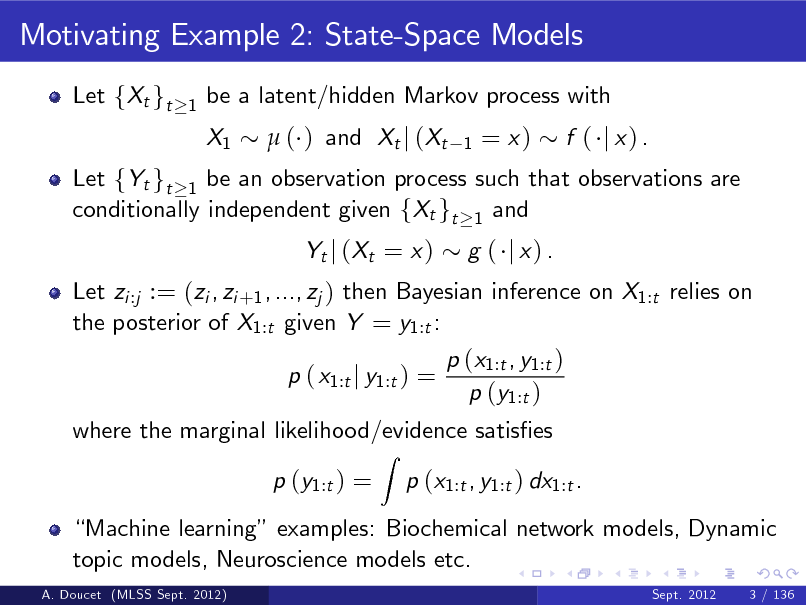
Motivating Example 2: State-Space Models
Let fXt gt
1
be a latent/hidden Markov process with X1 ( ) and Xt j (Xt
1
= x)
f ( j x) .
A. Doucet (MLSS Sept. 2012)
Sept. 2012
3 / 136
6
Motivating Example 2: State-Space Models
Let fXt gt
1
be a latent/hidden Markov process with X1 ( ) and Xt j (Xt
1
= x)
Let fYt gt 1 be an observation process such that observations are conditionally independent given fXt gt 1 and Yt j ( Xt = x ) g ( j x) .
f ( j x) .
A. Doucet (MLSS Sept. 2012)
Sept. 2012
3 / 136
7
Motivating Example 2: State-Space Models
Let fXt gt
1
be a latent/hidden Markov process with X1 ( ) and Xt j (Xt
1
= x)
Let fYt gt 1 be an observation process such that observations are conditionally independent given fXt gt 1 and Let zi :j := (zi , zi +1 , ..., zj ) then Bayesian inference on X1:t relies on the posterior of X1:t given Y = y1:t : p ( x1:t j y1:t ) =
Z
f ( j x) .
Yt j ( Xt = x )
g ( j x) .
p (x1:t , y1:t ) p (y1:t )
where the marginal likelihood/evidence satises p (y1:t ) = p (x1:t , y1:t ) dx1:t .
A. Doucet (MLSS Sept. 2012)
Sept. 2012
3 / 136
8
Motivating Example 2: State-Space Models
Let fXt gt
1
be a latent/hidden Markov process with X1 ( ) and Xt j (Xt
1
= x)
Let fYt gt 1 be an observation process such that observations are conditionally independent given fXt gt 1 and Let zi :j := (zi , zi +1 , ..., zj ) then Bayesian inference on X1:t relies on the posterior of X1:t given Y = y1:t : p ( x1:t j y1:t ) =
Z
f ( j x) .
Yt j ( Xt = x )
g ( j x) .
p (x1:t , y1:t ) p (y1:t )
where the marginal likelihood/evidence satises p (y1:t ) = p (x1:t , y1:t ) dx1:t .
Machine learning examples: Biochemical network models, Dynamic topic models, Neuroscience models etc.
A. Doucet (MLSS Sept. 2012) Sept. 2012 3 / 136
9

Bayesian Inference and Machine Learning
Bayesian approaches have been adopted by a large part of the ML community.
A. Doucet (MLSS Sept. 2012)
Sept. 2012
4 / 136
10

Bayesian Inference and Machine Learning
Bayesian approaches have been adopted by a large part of the ML community. Bayesian inference oers a number of attractive advantages over conventional approach
A. Doucet (MLSS Sept. 2012)
Sept. 2012
4 / 136
11
Bayesian Inference and Machine Learning
Bayesian approaches have been adopted by a large part of the ML community. Bayesian inference oers a number of attractive advantages over conventional approach
exibility in constructing complex models from simple parts;
A. Doucet (MLSS Sept. 2012)
Sept. 2012
4 / 136
12

Bayesian Inference and Machine Learning
Bayesian approaches have been adopted by a large part of the ML community. Bayesian inference oers a number of attractive advantages over conventional approach
exibility in constructing complex models from simple parts; the incorporation of prior knowledge is very natural;
A. Doucet (MLSS Sept. 2012)
Sept. 2012
4 / 136
13
Bayesian Inference and Machine Learning
Bayesian approaches have been adopted by a large part of the ML community. Bayesian inference oers a number of attractive advantages over conventional approach
exibility in constructing complex models from simple parts; the incorporation of prior knowledge is very natural; all modelling assumptions are made explicit;
A. Doucet (MLSS Sept. 2012)
Sept. 2012
4 / 136
14
Bayesian Inference and Machine Learning
Bayesian approaches have been adopted by a large part of the ML community. Bayesian inference oers a number of attractive advantages over conventional approach
exibility in constructing complex models from simple parts; the incorporation of prior knowledge is very natural; all modelling assumptions are made explicit; uncertainties over model order;
A. Doucet (MLSS Sept. 2012)
Sept. 2012
4 / 136
15
Bayesian Inference and Machine Learning
Bayesian approaches have been adopted by a large part of the ML community. Bayesian inference oers a number of attractive advantages over conventional approach
exibility in constructing complex models from simple parts; the incorporation of prior knowledge is very natural; all modelling assumptions are made explicit; uncertainties over model order; model parameters and predictions are technically straightforward to compute;
A. Doucet (MLSS Sept. 2012)
Sept. 2012
4 / 136
16
Bayesian Inference and Machine Learning
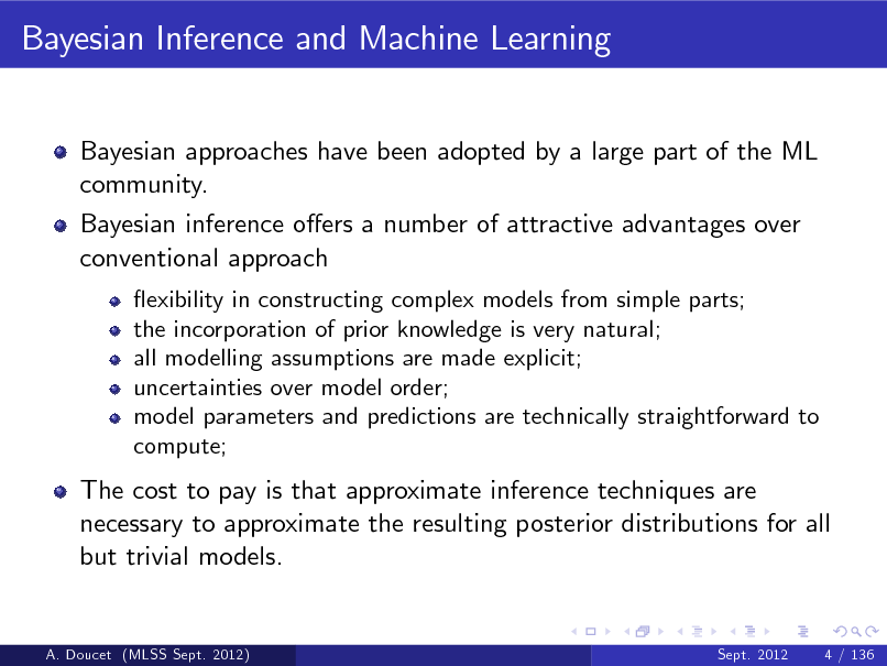
Bayesian approaches have been adopted by a large part of the ML community. Bayesian inference oers a number of attractive advantages over conventional approach
exibility in constructing complex models from simple parts; the incorporation of prior knowledge is very natural; all modelling assumptions are made explicit; uncertainties over model order; model parameters and predictions are technically straightforward to compute;
The cost to pay is that approximate inference techniques are necessary to approximate the resulting posterior distributions for all but trivial models.
A. Doucet (MLSS Sept. 2012)
Sept. 2012
4 / 136
17
Approximate Inference Methods
Gaussian/Laplace approximation, local linearization, Extended Kalman lters.
A. Doucet (MLSS Sept. 2012)
Sept. 2012
5 / 136
18
Approximate Inference Methods
Gaussian/Laplace approximation, local linearization, Extended Kalman lters. Variational methods, density assumed lters.
A. Doucet (MLSS Sept. 2012)
Sept. 2012
5 / 136
19
Approximate Inference Methods
Gaussian/Laplace approximation, local linearization, Extended Kalman lters. Variational methods, density assumed lters. Expectation-Propagation.
A. Doucet (MLSS Sept. 2012)
Sept. 2012
5 / 136
20
Approximate Inference Methods
Gaussian/Laplace approximation, local linearization, Extended Kalman lters. Variational methods, density assumed lters. Expectation-Propagation. Markov chain Monte Carlo (MCMC) methods.
A. Doucet (MLSS Sept. 2012)
Sept. 2012
5 / 136
21
Approximate Inference Methods
Gaussian/Laplace approximation, local linearization, Extended Kalman lters. Variational methods, density assumed lters. Expectation-Propagation. Markov chain Monte Carlo (MCMC) methods. Sequential Monte Carlo (SMC) methods.
A. Doucet (MLSS Sept. 2012)
Sept. 2012
5 / 136
22
Monte Carlo Methods
Variational and EP methods are computationally cheap but perform functional approximations of the posteriors of interest.
A. Doucet (MLSS Sept. 2012)
Sept. 2012
6 / 136
23
Monte Carlo Methods
Variational and EP methods are computationally cheap but perform functional approximations of the posteriors of interest. Both MCMC and SMC are asymptotically (as you increase computational eorts) bias-free but computationally expensive.
A. Doucet (MLSS Sept. 2012)
Sept. 2012
6 / 136
24
Monte Carlo Methods
Variational and EP methods are computationally cheap but perform functional approximations of the posteriors of interest. Both MCMC and SMC are asymptotically (as you increase computational eorts) bias-free but computationally expensive. MCMC are the tools of choice in Bayesian computation for over 20 years whereas SMC have been widely used for 15 years in vision and robotics.
A. Doucet (MLSS Sept. 2012)
Sept. 2012
6 / 136
25
Monte Carlo Methods
Variational and EP methods are computationally cheap but perform functional approximations of the posteriors of interest. Both MCMC and SMC are asymptotically (as you increase computational eorts) bias-free but computationally expensive. MCMC are the tools of choice in Bayesian computation for over 20 years whereas SMC have been widely used for 15 years in vision and robotics. The development of new methodology combined to the emergence of cheap multicore architectures makes now SMC a powerful alternative/complementary approach to MCMC to address general Bayesian computational problems.
A. Doucet (MLSS Sept. 2012)
Sept. 2012
6 / 136
26

Monte Carlo Methods
Variational and EP methods are computationally cheap but perform functional approximations of the posteriors of interest. Both MCMC and SMC are asymptotically (as you increase computational eorts) bias-free but computationally expensive. MCMC are the tools of choice in Bayesian computation for over 20 years whereas SMC have been widely used for 15 years in vision and robotics. The development of new methodology combined to the emergence of cheap multicore architectures makes now SMC a powerful alternative/complementary approach to MCMC to address general Bayesian computational problems. The aim of these lectures is to provide an introduction to this active research eld and discuss some open research problems.
A. Doucet (MLSS Sept. 2012)
Sept. 2012
6 / 136
27

Some References and Resources
A.D., J.F.G. De Freitas & N.J. Gordon (editors), Sequential Monte Carlo Methods in Practice, Springer-Verlag: New York, 2001.
A. Doucet (MLSS Sept. 2012)
Sept. 2012
7 / 136
28

Some References and Resources
A.D., J.F.G. De Freitas & N.J. Gordon (editors), Sequential Monte Carlo Methods in Practice, Springer-Verlag: New York, 2001. P. Del Moral, Feynman-Kac Formulae: Genealogical and Interacting Particle Systems with Applications, Springer-Verlag: New York, 2004.
A. Doucet (MLSS Sept. 2012)
Sept. 2012
7 / 136
29

Some References and Resources
A.D., J.F.G. De Freitas & N.J. Gordon (editors), Sequential Monte Carlo Methods in Practice, Springer-Verlag: New York, 2001. P. Del Moral, Feynman-Kac Formulae: Genealogical and Interacting Particle Systems with Applications, Springer-Verlag: New York, 2004. O. Capp, E. Moulines & T. Ryden, Hidden Markov Models, Springer-Verlag: New York, 2005.
A. Doucet (MLSS Sept. 2012)
Sept. 2012
7 / 136
30

Some References and Resources
A.D., J.F.G. De Freitas & N.J. Gordon (editors), Sequential Monte Carlo Methods in Practice, Springer-Verlag: New York, 2001. P. Del Moral, Feynman-Kac Formulae: Genealogical and Interacting Particle Systems with Applications, Springer-Verlag: New York, 2004. O. Capp, E. Moulines & T. Ryden, Hidden Markov Models, Springer-Verlag: New York, 2005. Webpage with links to papers and codes: http://www.stats.ox.ac.uk/~doucet/smc_resources.html
A. Doucet (MLSS Sept. 2012)
Sept. 2012
7 / 136
31

Some References and Resources
A.D., J.F.G. De Freitas & N.J. Gordon (editors), Sequential Monte Carlo Methods in Practice, Springer-Verlag: New York, 2001. P. Del Moral, Feynman-Kac Formulae: Genealogical and Interacting Particle Systems with Applications, Springer-Verlag: New York, 2004. O. Capp, E. Moulines & T. Ryden, Hidden Markov Models, Springer-Verlag: New York, 2005. Webpage with links to papers and codes: http://www.stats.ox.ac.uk/~doucet/smc_resources.html Thousands of papers on the subject appear every year.
A. Doucet (MLSS Sept. 2012)
Sept. 2012
7 / 136
32

Organization of Lectures
State-Space Models (approx.4 hours)
A. Doucet (MLSS Sept. 2012)
Sept. 2012
8 / 136
33

Organization of Lectures
State-Space Models (approx.4 hours)
SMC ltering and smoothing
A. Doucet (MLSS Sept. 2012)
Sept. 2012
8 / 136
34

Organization of Lectures
State-Space Models (approx.4 hours)
SMC ltering and smoothing Maximum likelihood parameter inference
A. Doucet (MLSS Sept. 2012)
Sept. 2012
8 / 136
35

Organization of Lectures
State-Space Models (approx.4 hours)
SMC ltering and smoothing Maximum likelihood parameter inference Bayesian parameter inference
A. Doucet (MLSS Sept. 2012)
Sept. 2012
8 / 136
36

Organization of Lectures
State-Space Models (approx.4 hours)
SMC ltering and smoothing Maximum likelihood parameter inference Bayesian parameter inference
Beyond State-Space Models (approx. 2 hours)
A. Doucet (MLSS Sept. 2012)
Sept. 2012
8 / 136
37

Organization of Lectures
State-Space Models (approx.4 hours)
SMC ltering and smoothing Maximum likelihood parameter inference Bayesian parameter inference
Beyond State-Space Models (approx. 2 hours)
SMC methods for generic sequence of target distributions
A. Doucet (MLSS Sept. 2012)
Sept. 2012
8 / 136
38

Organization of Lectures
State-Space Models (approx.4 hours)
SMC ltering and smoothing Maximum likelihood parameter inference Bayesian parameter inference
Beyond State-Space Models (approx. 2 hours)
SMC methods for generic sequence of target distributions SMC samplers.
A. Doucet (MLSS Sept. 2012)
Sept. 2012
8 / 136
39
Organization of Lectures
State-Space Models (approx.4 hours)
SMC ltering and smoothing Maximum likelihood parameter inference Bayesian parameter inference
Beyond State-Space Models (approx. 2 hours)
SMC methods for generic sequence of target distributions SMC samplers. Approximate Bayesian Computation.
A. Doucet (MLSS Sept. 2012)
Sept. 2012
8 / 136
40

Organization of Lectures
State-Space Models (approx.4 hours)
SMC ltering and smoothing Maximum likelihood parameter inference Bayesian parameter inference
Beyond State-Space Models (approx. 2 hours)
SMC methods for generic sequence of target distributions SMC samplers. Approximate Bayesian Computation. Optimal design, optimal control.
A. Doucet (MLSS Sept. 2012)
Sept. 2012
8 / 136
41

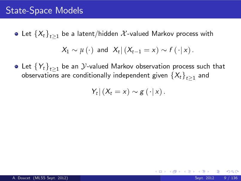
State-Space Models
Let fXt gt
1
be a latent/hidden X -valued Markov process with X1 ( ) and Xt j (Xt
1
= x)
f ( j x) .
A. Doucet (MLSS Sept. 2012)
Sept. 2012
9 / 136
42
State-Space Models
Let fXt gt
1
be a latent/hidden X -valued Markov process with X1 ( ) and Xt j (Xt
1
= x)
f ( j x) .
Let fYt gt 1 be an Y -valued Markov observation process such that observations are conditionally independent given fXt gt 1 and Yt j ( Xt = x ) g ( j x) .
A. Doucet (MLSS Sept. 2012)
Sept. 2012
9 / 136
43
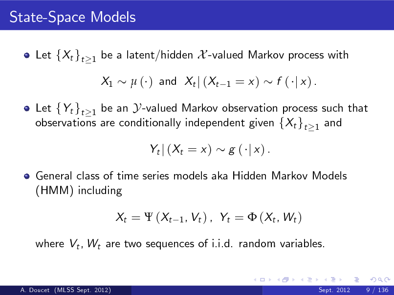
State-Space Models
Let fXt gt
1
be a latent/hidden X -valued Markov process with X1 ( ) and Xt j (Xt
1
= x)
f ( j x) .
Let fYt gt 1 be an Y -valued Markov observation process such that observations are conditionally independent given fXt gt 1 and Yt j ( Xt = x ) g ( j x) .
General class of time series models aka Hidden Markov Models (HMM) including Xt = ( Xt
1 , Vt ) ,
Yt = ( Xt , W t )
where Vt , Wt are two sequences of i.i.d. random variables.
A. Doucet (MLSS Sept. 2012)
Sept. 2012
9 / 136
44
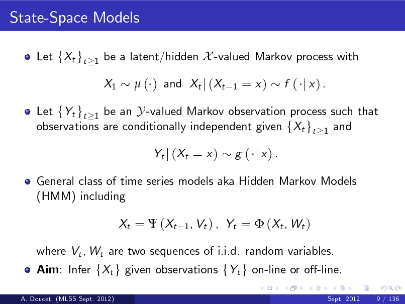
State-Space Models
Let fXt gt
1
be a latent/hidden X -valued Markov process with X1 ( ) and Xt j (Xt
1
= x)
f ( j x) .
Let fYt gt 1 be an Y -valued Markov observation process such that observations are conditionally independent given fXt gt 1 and Yt j ( Xt = x ) g ( j x) .
General class of time series models aka Hidden Markov Models (HMM) including Xt = ( Xt
1 , Vt ) ,
Yt = ( Xt , W t )
where Vt , Wt are two sequences of i.i.d. random variables. Aim: Infer fXt g given observations fYt g on-line or o-line.
A. Doucet (MLSS Sept. 2012) Sept. 2012 9 / 136
45

State-Space Models
State-space models are ubiquitous in control, data mining, econometrics, geosciences, system biology etc. Since Jan. 2012, more than 13,500 papers have already appeared (source: Google Scholar).
A. Doucet (MLSS Sept. 2012)
Sept. 2012
10 / 136
46

State-Space Models
State-space models are ubiquitous in control, data mining, econometrics, geosciences, system biology etc. Since Jan. 2012, more than 13,500 papers have already appeared (source: Google Scholar). Finite State-space HMM: X is a nite space, i.e. fXt g is a nite Markov chain Yt j ( Xt = x ) g ( j x )
A. Doucet (MLSS Sept. 2012)
Sept. 2012
10 / 136
47
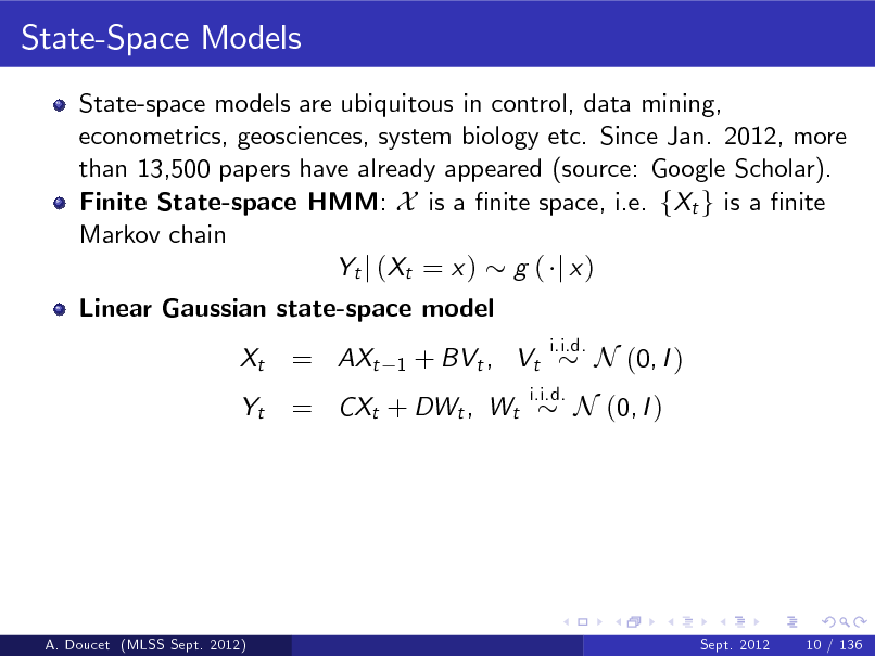
State-Space Models
State-space models are ubiquitous in control, data mining, econometrics, geosciences, system biology etc. Since Jan. 2012, more than 13,500 papers have already appeared (source: Google Scholar). Finite State-space HMM: X is a nite space, i.e. fXt g is a nite Markov chain Yt j ( Xt = x ) g ( j x ) Linear Gaussian state-space model Xt Yt
= AXt
1
+ BVt , Vt
i.i.d.
= CXt + DWt , Wt
i.i.d.
N (0, I )
N (0, I )
A. Doucet (MLSS Sept. 2012)
Sept. 2012
10 / 136
48
State-Space Models
State-space models are ubiquitous in control, data mining, econometrics, geosciences, system biology etc. Since Jan. 2012, more than 13,500 papers have already appeared (source: Google Scholar). Finite State-space HMM: X is a nite space, i.e. fXt g is a nite Markov chain Yt j ( Xt = x ) g ( j x ) Linear Gaussian state-space model Xt Yt
= AXt
1
+ BVt , Vt
i.i.d.
= CXt + DWt , Wt
i.i.d.
N (0, I )
Switching Linear Gaussian state-space model: Xt = Xt1 , Xt2 where Xt1 is a nite Markov chain, Xt2 = A Xt1 Xt2 Yt
1
N (0, I )
+ B Xt1 Vt , Vt
i.i.d.
= C Xt1 Xt2 + D Xt1 Wt , Wt
i.i.d.
N (0, I )
Sept. 2012 10 / 136
N (0, I )
A. Doucet (MLSS Sept. 2012)
49
State-Space Models
Stochastic Volatility model Xt Yt
i.i.d.
= Xt
1
+ Vt , Vt
= exp (Xt /2) Wt , Wt
i.i.d.
N (0, 1) N (0, 1)
A. Doucet (MLSS Sept. 2012)
Sept. 2012
11 / 136
50
State-Space Models
Stochastic Volatility model Xt Yt
i.i.d.
= Xt
1
+ Vt , Vt
= exp (Xt /2) Wt , Wt
i.i.d.
N (0, 1) N (0, 1)
Biochemical Network model Pr Xt1+dt =xt1+1, Xt2+dt =xt2 xt1 , xt2 = xt1 dt + o (dt ) , Pr Xt1+dt =xt1 1, Xt2+dt =xt2+1 xt1 , xt2 = xt1 xt2 dt + o (dt ) , Pr Xt1+dt =xt1 , Xt2+dt =xt2 1 xt1 , xt2 = xt2 dt + o (dt ) , with
1 Yk = Xk T + Wk with Wk i.i.d.
N 0, 2 .
A. Doucet (MLSS Sept. 2012)
Sept. 2012
11 / 136
51
State-Space Models
Stochastic Volatility model Xt Yt
i.i.d.
= Xt
1
+ Vt , Vt
= exp (Xt /2) Wt , Wt
i.i.d.
N (0, 1) N (0, 1)
Biochemical Network model Pr Xt1+dt =xt1+1, Xt2+dt =xt2 xt1 , xt2 = xt1 dt + o (dt ) , Pr Xt1+dt =xt1 1, Xt2+dt =xt2+1 xt1 , xt2 = xt1 xt2 dt + o (dt ) , Pr Xt1+dt =xt1 , Xt2+dt =xt2 1 xt1 , xt2 = xt2 dt + o (dt ) , with
1 Yk = Xk T + Wk with Wk i.i.d.
Nonlinear Diusion model dXt Yk
i.i.d.
N 0, 2 .
= (Xt ) dt + (Xt ) dVt , Vt Brownian motion = (Xk T ) +Wk , Wk N 0, 2 .
Sept. 2012 11 / 136
A. Doucet (MLSS Sept. 2012)
52
Inference in State-Space Models
Given observations y1:t := (y1 , y2 , . . . , yt ), inference about X1:t := (X1 , ..., Xt ) relies on the posterior p ( x1:t j y1:t ) = where p (x1:t , y1:t ) = (x1 ) f ( xk j xk p (y1:t ) =
Z
t 1) k =2
p (x1:t , y1:t ) p (y1:t )
|
Z
p (x1:t )
p (x1:t , y1:t ) dx1:t
{z
}k =1 {z |
g ( yk j xk ),
p ( y1:t jx1:t )
t
}
A. Doucet (MLSS Sept. 2012)
Sept. 2012
12 / 136
53
Inference in State-Space Models
Given observations y1:t := (y1 , y2 , . . . , yt ), inference about X1:t := (X1 , ..., Xt ) relies on the posterior p ( x1:t j y1:t ) = where p (x1:t , y1:t ) = (x1 ) f ( xk j xk p (y1:t ) =
Z
t 1) k =2
p (x1:t , y1:t ) p (y1:t )
|
When X is nite & linear Gaussian models, fp ( xt j y1:t )gt 1 can be computed exactly. For non-linear models, approximations are required: EKF, UKF, Gaussian sum lters, etc.
Z
p (x1:t )
p (x1:t , y1:t ) dx1:t
{z
}k =1 {z |
g ( yk j xk ),
p ( y1:t jx1:t )
t
}
A. Doucet (MLSS Sept. 2012)
Sept. 2012
12 / 136
54
Inference in State-Space Models
Given observations y1:t := (y1 , y2 , . . . , yt ), inference about X1:t := (X1 , ..., Xt ) relies on the posterior p ( x1:t j y1:t ) = where p (x1:t , y1:t ) = (x1 ) f ( xk j xk p (y1:t ) =
Z
t 1) k =2
p (x1:t , y1:t ) p (y1:t )
|
A. Doucet (MLSS Sept. 2012)
When X is nite & linear Gaussian models, fp ( xt j y1:t )gt 1 can be computed exactly. For non-linear models, approximations are required: EKF, UKF, Gaussian sum lters, etc. Approximations of fp ( xt j y1:t )gT=1 provide approximation of t p ( x1:T j y1:T ) .
Sept. 2012
Z
p (x1:t )
p (x1:t , y1:t ) dx1:t
{z
}k =1 {z |
g ( yk j xk ),
p ( y1:t jx1:t )
t
}
12 / 136
55
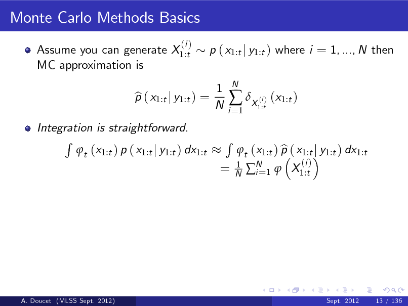
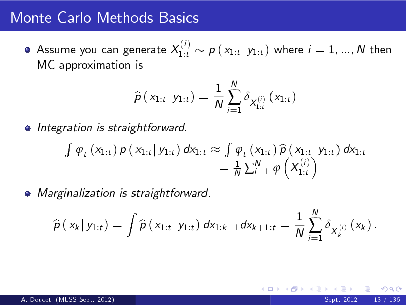
Monte Carlo Methods Basics
Assume you can generate X1:t MC approximation is
(i )
p ( x1:t j y1:t ) where i = 1, ..., N then 1 N
p ( x1:t j y1:t ) = b
i =1
X ( ) (x1:t )
i 1:t
N
A. Doucet (MLSS Sept. 2012)
Sept. 2012
13 / 136
56
Monte Carlo Methods Basics
Assume you can generate X1:t MC approximation is
(i )
p ( x1:t j y1:t ) where i = 1, ..., N then 1 N
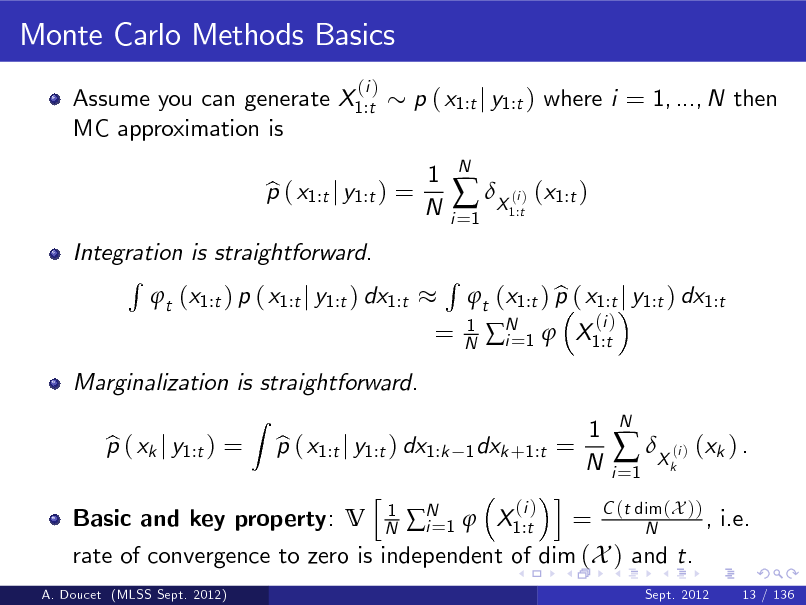
Integration is straightforward. R t (x1:t ) p ( x1:t j y1:t ) dx1:t
p ( x1:t j y1:t ) = b
i =1
X ( ) (x1:t )
i 1:t
N
=
R
1 N
b t (x1:t ) p ( x1:t j y1:t ) dx1:t N 1 X1:t i=
(i )
A. Doucet (MLSS Sept. 2012)
Sept. 2012
13 / 136
57
Monte Carlo Methods Basics
Assume you can generate X1:t MC approximation is
(i )
p ( x1:t j y1:t ) where i = 1, ..., N then 1 N
Integration is straightforward. R t (x1:t ) p ( x1:t j y1:t ) dx1:t
Z
p ( x1:t j y1:t ) = b
i =1
X ( ) (x1:t )
i 1:t
N
=
R
1 N
Marginalization is straightforward. p ( xk j y1:t ) = b p ( x1:t j y1:t ) dx1:k b
b t (x1:t ) p ( x1:t j y1:t ) dx1:t N 1 X1:t i=
(i )
1 dxk +1:t =
1 N
i =1
X ( ) (xk ) .
i k
N
A. Doucet (MLSS Sept. 2012)
Sept. 2012
13 / 136
58
Monte Carlo Methods Basics
Assume you can generate X1:t MC approximation is
(i )
p ( x1:t j y1:t ) where i = 1, ..., N then 1 N
Integration is straightforward. R t (x1:t ) p ( x1:t j y1:t ) dx1:t
Z
p ( x1:t j y1:t ) = b
i =1
X ( ) (x1:t )
i 1:t
N
=
R
1 N
Marginalization is straightforward. p ( xk j y1:t ) = b p ( x1:t j y1:t ) dx1:k b h
1 N
b t (x1:t ) p ( x1:t j y1:t ) dx1:t N 1 X1:t i=
(i )
1 dxk +1:t =
1 N
Basic and key property: V
A. Doucet (MLSS Sept. 2012)
i (i ) = C (t dim (X )) , i.e. N 1 X1:t i= N rate of convergence to zero is independent of dim (X ) and t.
Sept. 2012 13 / 136
i =1
X ( ) (xk ) .
i k
N
59
Monte Carlo Methods
Problem 1: We cannot typically generate exact samples from p ( x1:t j y1:t ) for non-linear non-Gaussian models.
A. Doucet (MLSS Sept. 2012)
Sept. 2012
14 / 136
60
Monte Carlo Methods
Problem 1: We cannot typically generate exact samples from p ( x1:t j y1:t ) for non-linear non-Gaussian models.
Problem 2: Even if we could, algorithms to generate samples from p ( x1:t j y1:t ) will have at least complexity O (t ) .
A. Doucet (MLSS Sept. 2012)
Sept. 2012
14 / 136
61
Monte Carlo Methods
Problem 1: We cannot typically generate exact samples from p ( x1:t j y1:t ) for non-linear non-Gaussian models.
Problem 2: Even if we could, algorithms to generate samples from p ( x1:t j y1:t ) will have at least complexity O (t ) . Typical solution to problem 1 is to generate approximate samples using MCMC methods but these methods are not recursive.
A. Doucet (MLSS Sept. 2012)
Sept. 2012
14 / 136
62
Monte Carlo Methods
Problem 1: We cannot typically generate exact samples from p ( x1:t j y1:t ) for non-linear non-Gaussian models.
Problem 2: Even if we could, algorithms to generate samples from p ( x1:t j y1:t ) will have at least complexity O (t ) . Typical solution to problem 1 is to generate approximate samples using MCMC methods but these methods are not recursive.
SMC Methods solves partially Problem 1 and Problem 2 by breaking the problem of sampling from p ( x1:t j y1:t ) into a collection of simpler subproblems. First approximate p ( x1 j y1 ) and p (y1 ) at time 1, then p ( x1:2 j y1:2 ) and p (y1:2 ) at time 2 and so on.
A. Doucet (MLSS Sept. 2012)
Sept. 2012
14 / 136
63
Monte Carlo Methods
Problem 1: We cannot typically generate exact samples from p ( x1:t j y1:t ) for non-linear non-Gaussian models.
Problem 2: Even if we could, algorithms to generate samples from p ( x1:t j y1:t ) will have at least complexity O (t ) . Typical solution to problem 1 is to generate approximate samples using MCMC methods but these methods are not recursive.
SMC Methods solves partially Problem 1 and Problem 2 by breaking the problem of sampling from p ( x1:t j y1:t ) into a collection of simpler subproblems. First approximate p ( x1 j y1 ) and p (y1 ) at time 1, then p ( x1:2 j y1:2 ) and p (y1:2 ) at time 2 and so on. Each target distribution is approximated by a cloud of random samples termed particles evolving according to importance sampling and resampling steps.
A. Doucet (MLSS Sept. 2012)
Sept. 2012
14 / 136
64

Standard Bayesian Recursion
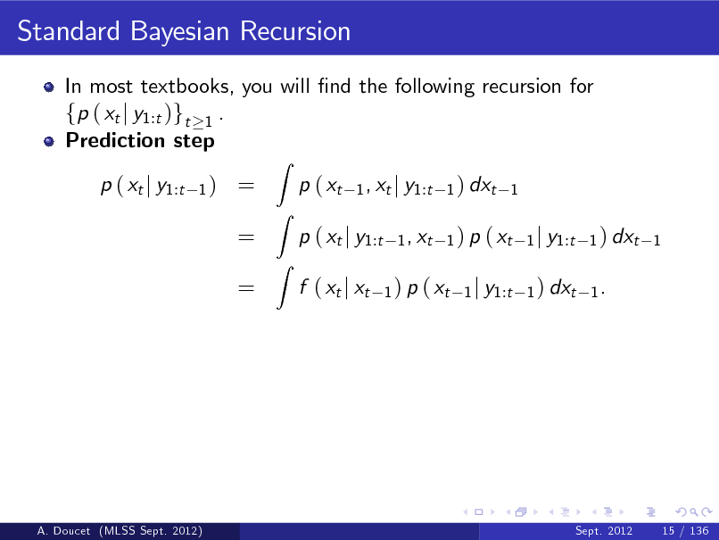
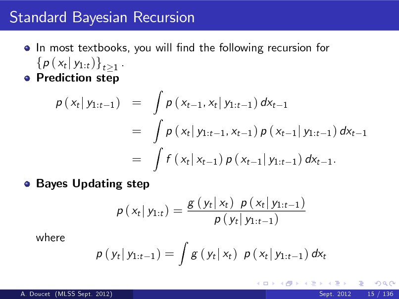
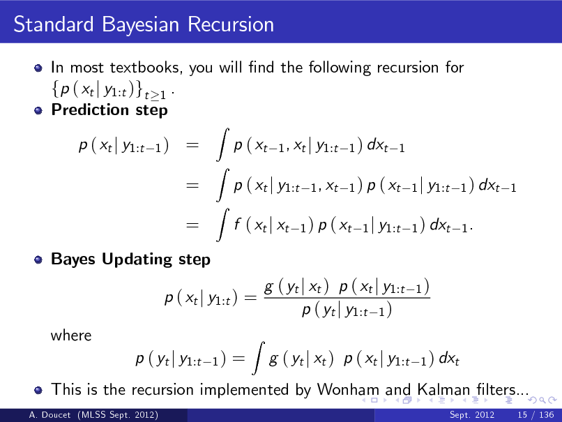
In most textbooks, you will nd the following recursion for fp ( xt j y1:t )gt 1 .
A. Doucet (MLSS Sept. 2012)
Sept. 2012
15 / 136
65
Standard Bayesian Recursion
In most textbooks, you will nd the following recursion for fp ( xt j y1:t )gt 1 . Prediction step p ( xt j y1:t
1)
= = =
Z
p ( xt
Z Z
1 , xt j y1:t 1 ) dxt 1 1 , xt 1 ) p ( xt 1 j y1:t 1 ) dxt 1 1 ) p ( xt 1 j y1:t 1 ) dxt 1 .
p ( xt j y1:t f ( xt j xt
A. Doucet (MLSS Sept. 2012)
Sept. 2012
15 / 136
66
Standard Bayesian Recursion
In most textbooks, you will nd the following recursion for fp ( xt j y1:t )gt 1 . Prediction step p ( xt j y1:t
1)
= = =
Z
p ( xt
Z Z
1 , xt j y1:t 1 ) dxt 1 1 , xt 1 ) p ( xt 1 j y1:t 1 ) dxt 1 1 ) p ( xt 1 j y1:t 1 ) dxt 1 .
p ( xt j y1:t f ( xt j xt
Bayes Updating step
p ( xt j y1:t ) = where p ( yt j y1:t
A. Doucet (MLSS Sept. 2012)
1)
=
Z
g ( yt j xt ) p ( xt j y1:t p ( yt j y1:t 1 ) g ( yt j xt ) p ( xt j y1:t
1)
1 ) dxt
Sept. 2012
15 / 136
67
Standard Bayesian Recursion
In most textbooks, you will nd the following recursion for fp ( xt j y1:t )gt 1 . Prediction step p ( xt j y1:t
1)
= = =
Z
p ( xt
Z Z
1 , xt j y1:t 1 ) dxt 1 1 , xt 1 ) p ( xt 1 j y1:t 1 ) dxt 1 1 ) p ( xt 1 j y1:t 1 ) dxt 1 .
p ( xt j y1:t f ( xt j xt
Bayes Updating step
p ( xt j y1:t ) = where p ( yt j y1:t
A. Doucet (MLSS Sept. 2012)
1)
=
This is the recursion implemented by Wonham and Kalman lters...
Sept. 2012 15 / 136
Z
g ( yt j xt ) p ( xt j y1:t p ( yt j y1:t 1 ) g ( yt j xt ) p ( xt j y1:t
1)
1 ) dxt
68
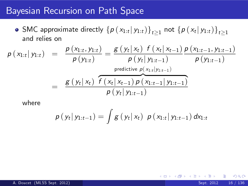
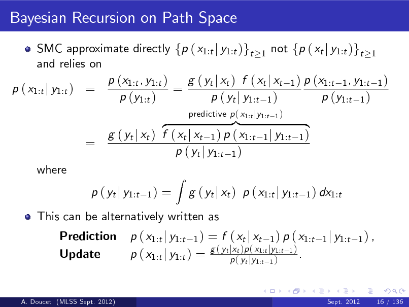
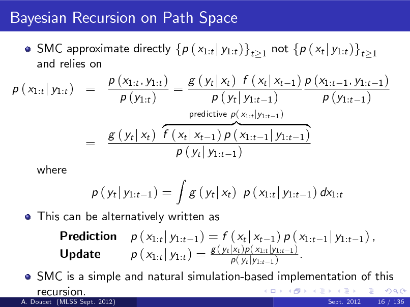
Bayesian Recursion on Path Space
SMC approximate directly fp ( x1:t j y1:t )gt 1 not fp ( xt j y1:t )gt 1 and relies on p (x1:t , y1:t ) g ( yt j xt ) f ( xt j xt 1 ) p (x1:t 1 , y1:t 1 ) p ( x1:t j y1:t ) = = p (y1:t ) p ( yt j y1:t 1 ) p (y1:t 1 )
=
where
}| z g ( yt j xt ) f ( xt j xt 1 ) p ( x1:t p ( yt j y1:t 1 )
1)
predictive p ( x1:t jy1:t
1)
1 j y1:t
{ 1)
1 ) dx1:t
p ( yt j y1:t
=
Z
g ( yt j xt ) p ( x1:t j y1:t
A. Doucet (MLSS Sept. 2012)
Sept. 2012
16 / 136
69
Bayesian Recursion on Path Space
SMC approximate directly fp ( x1:t j y1:t )gt 1 not fp ( xt j y1:t )gt 1 and relies on p (x1:t , y1:t ) g ( yt j xt ) f ( xt j xt 1 ) p (x1:t 1 , y1:t 1 ) p ( x1:t j y1:t ) = = p (y1:t ) p ( yt j y1:t 1 ) p (y1:t 1 )
=
where
}| z g ( yt j xt ) f ( xt j xt 1 ) p ( x1:t p ( yt j y1:t 1 )
1)
predictive p ( x1:t jy1:t
1)
1 j y1:t
{ 1)
1 ) dx1:t
p ( yt j y1:t Prediction Update
=
This can be alternatively written as p ( x1:t j y1:t 1 ) = f ( xt j xt 1 ) p ( x1:t g ( yt jxt )p ( x1:t jy1:t 1 ) . p ( x1:t j y1:t ) = p ( yt jy1:t 1 )
1 j y1:t 1 ) ,
Z
g ( yt j xt ) p ( x1:t j y1:t
A. Doucet (MLSS Sept. 2012)
Sept. 2012
16 / 136
70
Bayesian Recursion on Path Space
SMC approximate directly fp ( x1:t j y1:t )gt 1 not fp ( xt j y1:t )gt 1 and relies on p (x1:t , y1:t ) g ( yt j xt ) f ( xt j xt 1 ) p (x1:t 1 , y1:t 1 ) p ( x1:t j y1:t ) = = p (y1:t ) p ( yt j y1:t 1 ) p (y1:t 1 )
=
where
}| z g ( yt j xt ) f ( xt j xt 1 ) p ( x1:t p ( yt j y1:t 1 )
1)
predictive p ( x1:t jy1:t
1)
1 j y1:t
{ 1)
1 ) dx1:t
p ( yt j y1:t Prediction Update
=
This can be alternatively written as p ( x1:t j y1:t 1 ) = f ( xt j xt 1 ) p ( x1:t g ( yt jxt )p ( x1:t jy1:t 1 ) . p ( x1:t j y1:t ) = p ( yt jy1:t 1 )
1 j y1:t 1 ) ,
Z
g ( yt j xt ) p ( x1:t j y1:t
SMC is a simple and natural simulation-based implementation of this recursion.
A. Doucet (MLSS Sept. 2012) Sept. 2012 16 / 136
71
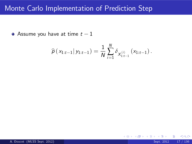
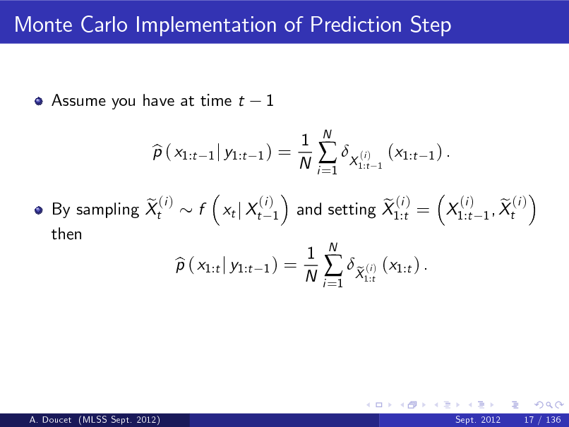
Monte Carlo Implementation of Prediction Step
Assume you have at time t p ( x1:t b
1
1 j y1:t 1 )
=
1 N
i =1
X ( )
N
i 1:t 1
(x1:t
1) .
A. Doucet (MLSS Sept. 2012)
Sept. 2012
17 / 136
72
Monte Carlo Implementation of Prediction Step
Assume you have at time t p ( x1:t b
1
1 j y1:t 1 )
=
1 N
i =1
X ( )
N
i 1:t 1
(x1:t
1) .
e (i ) By sampling Xt then
f
xt j Xt
(i ) 1
p ( x1:t j y1:t b
1)
=
(i ) e (i ) e (i ) and setting X1:t = X1:t 1 , Xt
1 N
i =1
X ( ) (x1:t ) . e
i 1:t
N
A. Doucet (MLSS Sept. 2012)
Sept. 2012
17 / 136
73
Monte Carlo Implementation of Prediction Step
Assume you have at time t p ( x1:t b
1
1 j y1:t 1 )
=
1 N
i =1
X ( )
N
i 1:t 1
(x1:t
1) .
e (i ) By sampling Xt then
f
xt j Xt
(i ) 1
Sampling from f ( xt j xt 1 ) is usually straightforward and can be done even if f ( xt j xt 1 ) does not admit any analytical expression; e.g. biochemical network models.
p ( x1:t j y1:t b
1)
=
(i ) e (i ) e (i ) and setting X1:t = X1:t 1 , Xt
1 N
i =1
X ( ) (x1:t ) . e
i 1:t
N
A. Doucet (MLSS Sept. 2012)
Sept. 2012
17 / 136
74
Importance Sampling Implementation of Updating Step
Our target at time t is p ( x1:t j y1:t ) = so by substituting p ( x1:t j y1:t b p ( yt j y1:t b
1)
g ( yt j xt ) p ( x1:t j y1:t p ( yt j y1:t 1 )
1)
1)
= =
Z
to p ( x1:t j y1:t
1)
we obtain
1 ) dx1:t
1 N
g ( yt j xt ) p ( x1:t j y1:t b
i =1
g
N
e (i ) . yt j Xt
A. Doucet (MLSS Sept. 2012)
Sept. 2012
18 / 136
75
Importance Sampling Implementation of Updating Step
Our target at time t is p ( x1:t j y1:t ) = so by substituting p ( x1:t j y1:t b p ( yt j y1:t b
1)
g ( yt j xt ) p ( x1:t j y1:t p ( yt j y1:t 1 )
1)
1)
= =
Z
to p ( x1:t j y1:t
1)
we obtain
1 ) dx1:t
1 N
g ( yt j xt ) p ( x1:t j y1:t b
i =1
g
N
We now have p ( x1:t j y1:t ) = e
(i )
e (i ) . yt j Xt
1)
with Wt
g
A. Doucet (MLSS Sept. 2012)
e (i ) , N 1 Wt(i ) = 1. yt j Xt i=
g ( yt j xt ) p ( x1:t j y1:t b p ( yt j y1:t 1 ) b
=
i =1
Wt
N
(i )
X (i ) (x1:t ) . e
1:t Sept. 2012 18 / 136
76
Multinomial Resampling
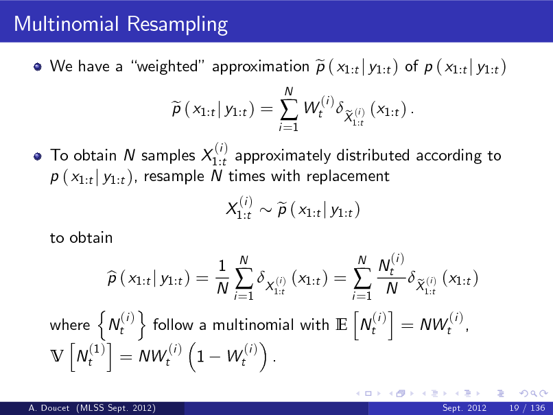
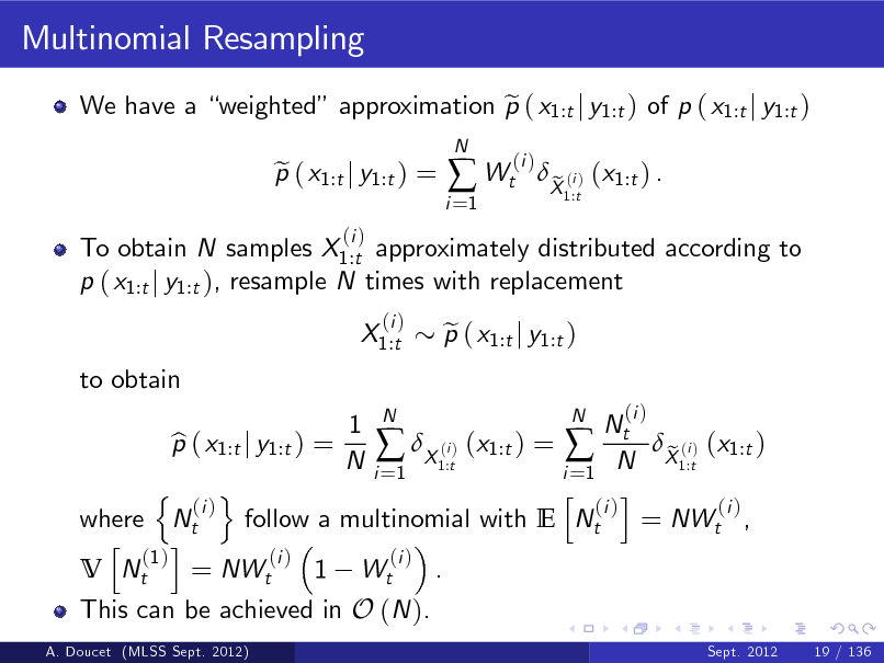
We have a weighted approximation p ( x1:t j y1:t ) of p ( x1:t j y1:t ) e p ( x1:t j y1:t ) = e
i =1 N
Wt
(i )
X (i ) (x1:t ) . e
1:t
A. Doucet (MLSS Sept. 2012)
Sept. 2012
19 / 136
77
Multinomial Resampling
We have a weighted approximation p ( x1:t j y1:t ) of p ( x1:t j y1:t ) e To obtain N samples X1:t approximately distributed according to p ( x1:t j y1:t ), resample N times with replacement X1:t to obtain
(i )
N
p ( x1:t j y1:t ) = e
(i )
i =1
Wt
(i )
X (i ) (x1:t ) . e
1:t
N 1 N Nt p ( x1:t j y1:t ) = b (i X1:t) (x1:t ) = N X1:t) (x1:t ) e (i N i =1 i =1 n o h i (i ) (i ) (i ) where Nt follow a multinomial with E Nt = NWt , h i (1 ) (i ) (i ) V Nt = NWt 1 Wt .
A. Doucet (MLSS Sept. 2012) Sept. 2012 19 / 136
p ( x1:t j y1:t ) e
(i )
78
Multinomial Resampling
We have a weighted approximation p ( x1:t j y1:t ) of p ( x1:t j y1:t ) e To obtain N samples X1:t approximately distributed according to p ( x1:t j y1:t ), resample N times with replacement X1:t to obtain
(i )
N
p ( x1:t j y1:t ) = e
(i )
i =1
Wt
(i )
X (i ) (x1:t ) . e
1:t
This can be achieved in O (N ).
A. Doucet (MLSS Sept. 2012)
N 1 N Nt p ( x1:t j y1:t ) = b (i X1:t) (x1:t ) = N X1:t) (x1:t ) e (i N i =1 i =1 n o h i (i ) (i ) (i ) where Nt follow a multinomial with E Nt = NWt , h i (1 ) (i ) (i ) V Nt = NWt 1 Wt .
Sept. 2012 19 / 136
p ( x1:t j y1:t ) e
(i )
79
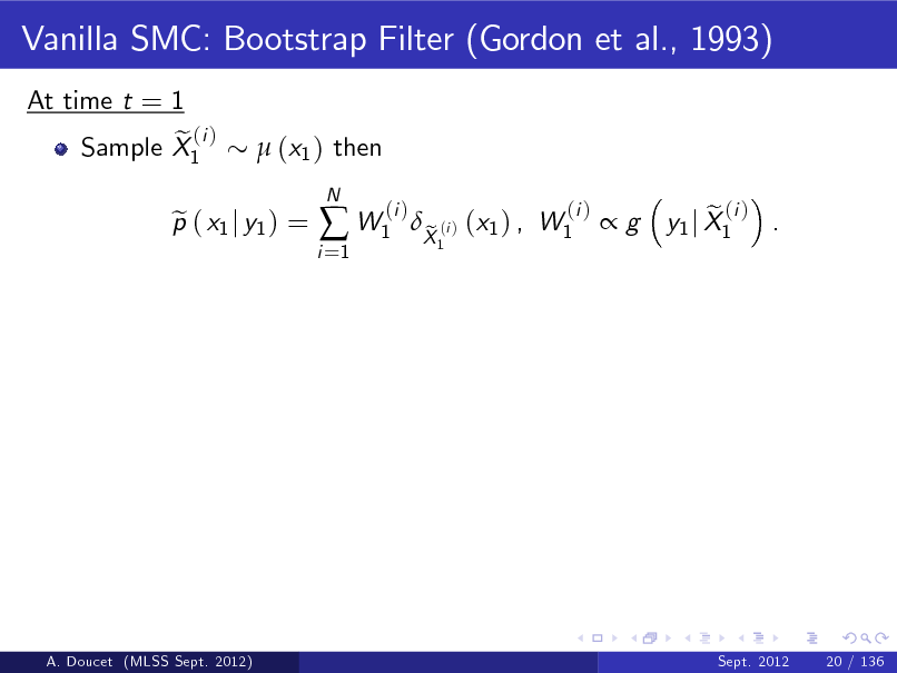
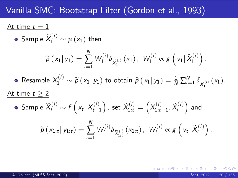
Vanilla SMC: Bootstrap Filter (Gordon et al., 1993)
At time t = 1 e (i ) Sample X1 (x1 ) then
p ( x1 j y1 ) = e
i =1
W1
N
(i )
X (i ) (x1 ) , W1 e
1
(i )
g
e (i ) y1 j X1 .
A. Doucet (MLSS Sept. 2012)
Sept. 2012
20 / 136
80

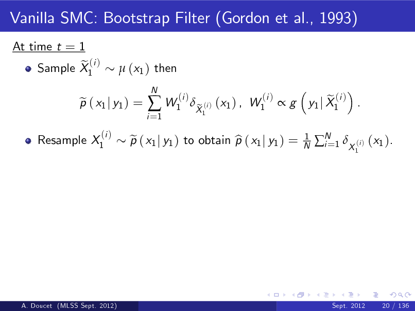
Vanilla SMC: Bootstrap Filter (Gordon et al., 1993)
At time t = 1 e (i ) Sample X1 (x1 ) then
Resample X1
p ( x1 j y1 ) = e
(i )
i =1
W1
N
(i )
p ( x1 j y1 ) to obtain p ( x1 j y1 ) = e b
X (i ) (x1 ) , W1 e
1
(i )
g
1 N
e (i ) y1 j X1 .
1
N 1 X (i ) (x1 ). i=
A. Doucet (MLSS Sept. 2012)
Sept. 2012
20 / 136
81
Vanilla SMC: Bootstrap Filter (Gordon et al., 1993)
At time t = 1 e (i ) Sample X1 (x1 ) then
Resample X1
p ( x1 j y1 ) = e
(i )
i =1
W1
N
(i )
p ( x1 j y1 ) to obtain p ( x1 j y1 ) = e b
X (i ) (x1 ) , W1 e
1
(i )
g
1 N
e (i ) y1 j X1 .
1
N 1 X (i ) (x1 ). i=
A. Doucet (MLSS Sept. 2012)
Sept. 2012
20 / 136
82
Vanilla SMC: Bootstrap Filter (Gordon et al., 1993)
At time t = 1 e (i ) Sample X1 (x1 ) then
Resample X1 At time t 2 e (i ) Sample Xt
p ( x1 j y1 ) = e
(i )
i =1
W1
N
(i )
p ( x1 j y1 ) to obtain p ( x1 j y1 ) = e b xt j Xt
N
X (i ) (x1 ) , W1 e
1
(i )
g
1 N
e (i ) y1 j X1 .
1
N 1 X (i ) (x1 ). i= and
f
(i ) 1
p ( x1:t j y1:t ) = e
i =1
Wt
(i )
(i ) e (i ) e (i ) , set X1:t = X1:t 1 , Xt
X (i ) (x1:t ) , Wt e
1:t
(i )
g
e (i ) . yt j Xt
A. Doucet (MLSS Sept. 2012)
Sept. 2012
20 / 136
83
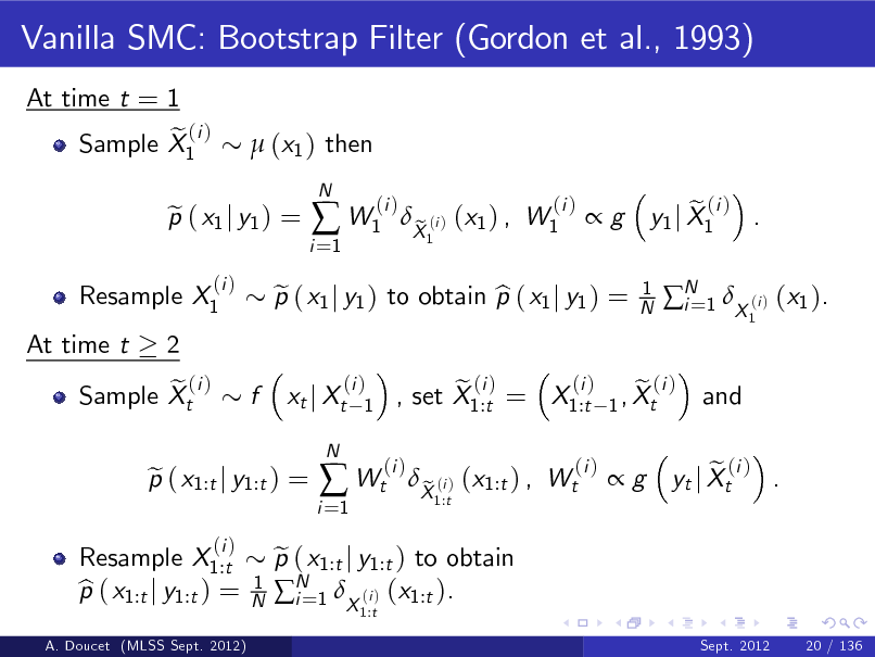
Vanilla SMC: Bootstrap Filter (Gordon et al., 1993)
At time t = 1 e (i ) Sample X1 (x1 ) then
Resample X1 At time t 2 e (i ) Sample Xt
p ( x1 j y1 ) = e
(i )
i =1
W1
N
(i )
p ( x1 j y1 ) to obtain p ( x1 j y1 ) = e b xt j Xt
N
X (i ) (x1 ) , W1 e
1
(i )
g
1 N
e (i ) y1 j X1 .
1
N 1 X (i ) (x1 ). i= and
f
(i ) 1
A. Doucet (MLSS Sept. 2012)
Resample X1:t p ( x1:t j y1:t ) = b
p ( x1:t j y1:t ) = e
(i )
1 N
i =1
Wt
(i )
(i ) e (i ) e (i ) , set X1:t = X1:t 1 , Xt
p ( x1:t j y1:t ) to obtain e N 1 X (i ) (x1:t ). i=
1:t
X (i ) (x1:t ) , Wt e
1:t
(i )
g
e (i ) . yt j Xt
Sept. 2012
20 / 136
84
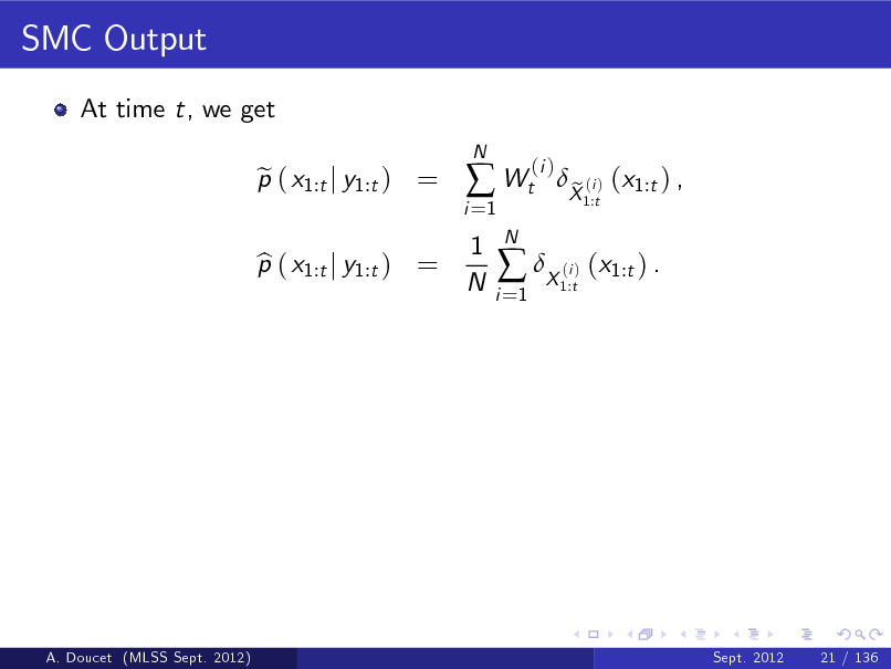
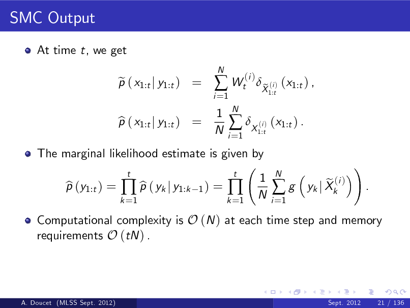
SMC Output
At time t, we get p ( x1:t j y1:t ) = e
N
i =1
Wt
1 N
N i =1
(i )
p ( x1:t j y1:t ) = b
X ( ) (x1:t ) .
i 1:t
X (i ) (x1:t ) , e
1:t
A. Doucet (MLSS Sept. 2012)
Sept. 2012
21 / 136
85
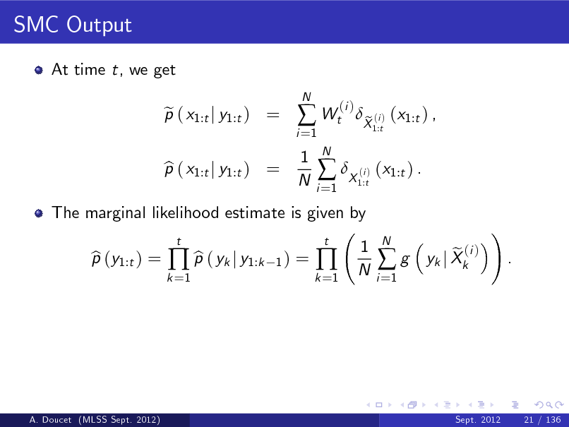
SMC Output
At time t, we get p ( x1:t j y1:t ) = e
N
i =1
Wt
1 N
N i =1
(i )
The marginal likelihood estimate is given by p (y1:t ) = b b p ( yk j y1:k
t 1)
p ( x1:t j y1:t ) = b
X ( ) (x1:t ) .
i 1:t
X (i ) (x1:t ) , e
1:t
=
k =1
k =1
t
1 N
i =1
g
N
e (i ) yk j Xk
!
.
A. Doucet (MLSS Sept. 2012)
Sept. 2012
21 / 136
86
SMC Output
At time t, we get p ( x1:t j y1:t ) = e
N
i =1
Wt
1 N
N i =1
(i )
The marginal likelihood estimate is given by p (y1:t ) = b b p ( yk j y1:k
t 1)
p ( x1:t j y1:t ) = b
X ( ) (x1:t ) .
i 1:t
X (i ) (x1:t ) , e
1:t
=
k =1
k =1
t
1 N
i =1
g
N
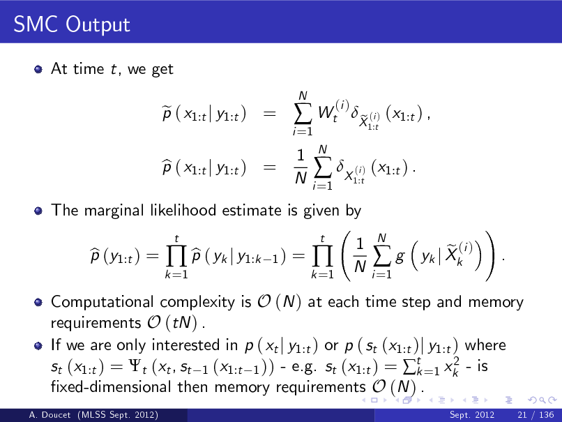
Computational complexity is O (N ) at each time step and memory requirements O (tN ) .
e (i ) yk j Xk
!
.
A. Doucet (MLSS Sept. 2012)
Sept. 2012
21 / 136
87
SMC Output
At time t, we get p ( x1:t j y1:t ) = e
N
i =1
Wt
1 N
N i =1
(i )
The marginal likelihood estimate is given by p (y1:t ) = b b p ( yk j y1:k
t 1)
p ( x1:t j y1:t ) = b
X ( ) (x1:t ) .
i 1:t
X (i ) (x1:t ) , e
1:t
=
k =1
k =1
t
1 N
i =1
g
N
Computational complexity is O (N ) at each time step and memory requirements O (tN ) . If we are only interested in p ( xt j y1:t ) or p ( st (x1:t )j y1:t ) where 2 st (x1:t ) = t (xt , st 1 (x1:t 1 )) - e.g. st (x1:t ) = t =1 xk - is k xed-dimensional then memory requirements O (N ) .
A. Doucet (MLSS Sept. 2012) Sept. 2012 21 / 136
e (i ) yk j Xk
!
.
88
![Slide: SMC on Path-Space - gures by Olivier Capp e
1.6 1.4 1.2
state
1 0.8 0.6 0.4
5
10 time index
15
20
25
1.6 1.4 1.2
state
1 0.8 0.6 0.4
5
10 time index
15
20
25
b Figure: p ( x1 j y1 ) and E [ X1 j y1 ] (top) and particle approximation of p ( x1 j y1 ) (bottom) (MLSS Sept. 2012) A. Doucet Sept. 2012 22 / 136](https://yosinski.com/mlss12/media/slides/MLSS-2012-Doucet-Sequential-Monte-Carlo-Methods_089.png)
SMC on Path-Space - gures by Olivier Capp e
1.6 1.4 1.2
state
1 0.8 0.6 0.4
5
10 time index
15
20
25
1.6 1.4 1.2
state
1 0.8 0.6 0.4
5
10 time index
15
20
25
b Figure: p ( x1 j y1 ) and E [ X1 j y1 ] (top) and particle approximation of p ( x1 j y1 ) (bottom) (MLSS Sept. 2012) A. Doucet Sept. 2012 22 / 136
89
![Slide: 1.6 1.4 1.2
state
1 0.8 0.6 0.4
5
10 time index
15
20
25
1.6 1.4 1.2
state
1 0.8 0.6 0.4
5
10 time index
15
20
25
b b Figure: p ( x1 j y1 ) , p ( x2 j y1 :2 )and E [ X1 j y1 ] , E [ X2 j y1 :2 ] (top) and particle approximation of p ( x1 :2 j y1 :2 ) (bottom)
A. Doucet (MLSS Sept. 2012) Sept. 2012 23 / 136](https://yosinski.com/mlss12/media/slides/MLSS-2012-Doucet-Sequential-Monte-Carlo-Methods_090.png)
1.6 1.4 1.2
state
1 0.8 0.6 0.4
5
10 time index
15
20
25
1.6 1.4 1.2
state
1 0.8 0.6 0.4
5
10 time index
15
20
25
b b Figure: p ( x1 j y1 ) , p ( x2 j y1 :2 )and E [ X1 j y1 ] , E [ X2 j y1 :2 ] (top) and particle approximation of p ( x1 :2 j y1 :2 ) (bottom)
A. Doucet (MLSS Sept. 2012) Sept. 2012 23 / 136
90
![Slide: 1.6 1.4 1.2
state
1 0.8 0.6 0.4
5
10 time index
15
20
25
1.6 1.4 1.2
state
1 0.8 0.6 0.4
5
10 time index
15
20
25
b Figure: p ( xt j y1 :t ) and E [ Xt j y1 :t ] for t = 1, 2, 3 (top) and particle approximation of p ( x1 :3 j y1 :3 ) (bottom)
A. Doucet (MLSS Sept. 2012) Sept. 2012 24 / 136](https://yosinski.com/mlss12/media/slides/MLSS-2012-Doucet-Sequential-Monte-Carlo-Methods_091.png)
1.6 1.4 1.2
state
1 0.8 0.6 0.4
5
10 time index
15
20
25
1.6 1.4 1.2
state
1 0.8 0.6 0.4
5
10 time index
15
20
25
b Figure: p ( xt j y1 :t ) and E [ Xt j y1 :t ] for t = 1, 2, 3 (top) and particle approximation of p ( x1 :3 j y1 :3 ) (bottom)
A. Doucet (MLSS Sept. 2012) Sept. 2012 24 / 136
91
![Slide: 1.6 1.4 1.2
state
1 0.8 0.6 0.4
5
10 time index
15
20
25
1.6 1.4 1.2
state
1 0.8 0.6 0.4
5
10 time index
15
20
25
b Figure: p ( xt j y1 :t ) and E [ Xt j y1 :t ] for t = 1, ..., 10 (top) and particle approximation of p ( x1 :10 j y1 :10 ) (bottom)
A. Doucet (MLSS Sept. 2012) Sept. 2012 25 / 136](https://yosinski.com/mlss12/media/slides/MLSS-2012-Doucet-Sequential-Monte-Carlo-Methods_092.png)
1.6 1.4 1.2
state
1 0.8 0.6 0.4
5
10 time index
15
20
25
1.6 1.4 1.2
state
1 0.8 0.6 0.4
5
10 time index
15
20
25
b Figure: p ( xt j y1 :t ) and E [ Xt j y1 :t ] for t = 1, ..., 10 (top) and particle approximation of p ( x1 :10 j y1 :10 ) (bottom)
A. Doucet (MLSS Sept. 2012) Sept. 2012 25 / 136
92
![Slide: 1.6 1.4 1.2
state
1 0.8 0.6 0.4
5
10 time index
15
20
25
1.6 1.4 1.2
state
1 0.8 0.6 0.4
5
10 time index
15
20
25
b Figure: p ( xt j y1 :t ) and E [ Xt j y1 :t ] for t = 1, ..., 24 (top) and particle approximation of p ( x1 :24 j y1 :24 ) (bottom)
A. Doucet (MLSS Sept. 2012) Sept. 2012 26 / 136](https://yosinski.com/mlss12/media/slides/MLSS-2012-Doucet-Sequential-Monte-Carlo-Methods_093.png)
1.6 1.4 1.2
state
1 0.8 0.6 0.4
5
10 time index
15
20
25
1.6 1.4 1.2
state
1 0.8 0.6 0.4
5
10 time index
15
20
25
b Figure: p ( xt j y1 :t ) and E [ Xt j y1 :t ] for t = 1, ..., 24 (top) and particle approximation of p ( x1 :24 j y1 :24 ) (bottom)
A. Doucet (MLSS Sept. 2012) Sept. 2012 26 / 136
93

Remarks
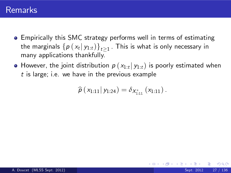
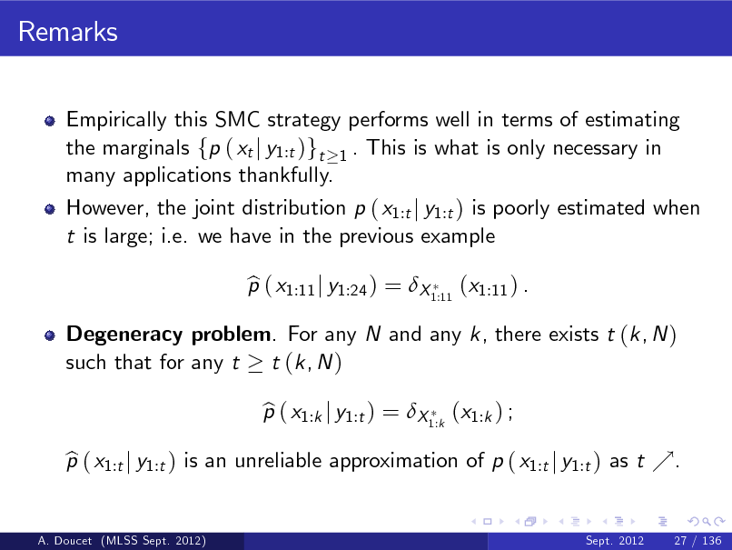
Empirically this SMC strategy performs well in terms of estimating the marginals fp ( xt j y1:t )gt 1 . This is what is only necessary in many applications thankfully.
A. Doucet (MLSS Sept. 2012)
Sept. 2012
27 / 136
94
Remarks
Empirically this SMC strategy performs well in terms of estimating the marginals fp ( xt j y1:t )gt 1 . This is what is only necessary in many applications thankfully. However, the joint distribution p ( x1:t j y1:t ) is poorly estimated when t is large; i.e. we have in the previous example p ( x1:11 j y1:24 ) = X 1:11 (x1:11 ) . b
A. Doucet (MLSS Sept. 2012)
Sept. 2012
27 / 136
95
Remarks
Empirically this SMC strategy performs well in terms of estimating the marginals fp ( xt j y1:t )gt 1 . This is what is only necessary in many applications thankfully. However, the joint distribution p ( x1:t j y1:t ) is poorly estimated when t is large; i.e. we have in the previous example p ( x1:11 j y1:24 ) = X 1:11 (x1:11 ) . b p ( x1:k j y1:t ) = X 1:k (x1:k ) ; b
Degeneracy problem. For any N and any k, there exists t (k, N ) such that for any t t (k, N )
p ( x1:t j y1:t ) is an unreliable approximation of p ( x1:t j y1:t ) as t %. b
A. Doucet (MLSS Sept. 2012) Sept. 2012 27 / 136
96
Another Illustration of the Degeneracy Phenomenon
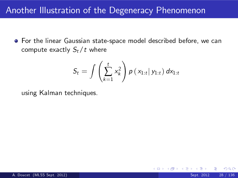
For the linear Gaussian state-space model described before, we can compute exactly St /t where ! Z St =
k =1
xk2
t
p ( x1:t j y1:t ) dx1:t
using Kalman techniques.
A. Doucet (MLSS Sept. 2012)
Sept. 2012
28 / 136
97
Another Illustration of the Degeneracy Phenomenon
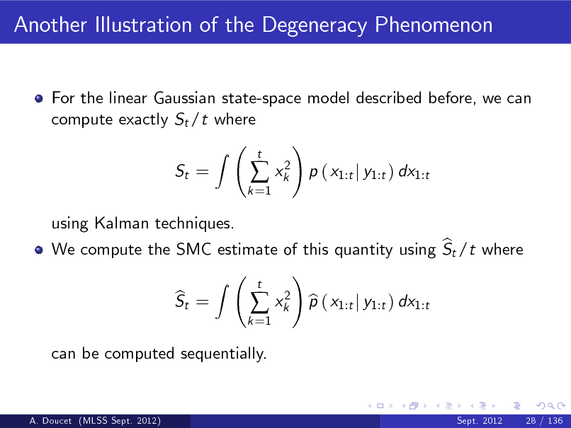
For the linear Gaussian state-space model described before, we can compute exactly St /t where ! Z St =
k =1
xk2
t
p ( x1:t j y1:t ) dx1:t
using Kalman techniques. b We compute the SMC estimate of this quantity using St /t where ! Z t 2 b St = b xk p ( x1:t j y1:t ) dx1:t
k =1
can be computed sequentially.
A. Doucet (MLSS Sept. 2012)
Sept. 2012
28 / 136
98
Another Illustration of the Degeneracy Phenomenon
0 .7
0 .6
0 .5
0 .4
0 .3
0 .2
0 .1
0
0
5 00
10 00
10 50
20 00
20 50
30 00
30 50
40 00
40 50
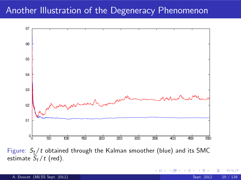
50 00
Figure: St /t obtained through the Kalman smoother (blue) and its SMC b estimate St /t (red).
A. Doucet (MLSS Sept. 2012)
Sept. 2012
29 / 136
99

Some Convergence Results for SMC
Numerous convergence results for SMC are available; see (Del Moral, 2004).
A. Doucet (MLSS Sept. 2012)
Sept. 2012
30 / 136
100
Some Convergence Results for SMC
Numerous convergence results for SMC are available; see (Del Moral, 2004). Let t : X t ! R and consider t = bt =
Z Z
t (x1:t ) p ( x1:t j y1:t ) dx1:t , b t (x1:t ) p ( x1:t j y1:t ) dx1:t = 1 N
i =1
t
N
X1:t .
(i )
A. Doucet (MLSS Sept. 2012)
Sept. 2012
30 / 136
101
![Slide: Some Convergence Results for SMC
Numerous convergence results for SMC are available; see (Del Moral, 2004). Let t : X t ! R and consider t = bt =
Z Z
t (x1:t ) p ( x1:t j y1:t ) dx1:t , b t (x1:t ) p ( x1:t j y1:t ) dx1:t = 1 N
i =1
t
N
X1:t . 1
(i )
We can prove that for any bounded function and any p B (t ) c (p ) k k 1/p p E [j b t t jp ] , N p lim N ( b t t ) ) N 0, 2 . t
N !
A. Doucet (MLSS Sept. 2012)
Sept. 2012
30 / 136](https://yosinski.com/mlss12/media/slides/MLSS-2012-Doucet-Sequential-Monte-Carlo-Methods_102.png)
Some Convergence Results for SMC
Numerous convergence results for SMC are available; see (Del Moral, 2004). Let t : X t ! R and consider t = bt =
Z Z
t (x1:t ) p ( x1:t j y1:t ) dx1:t , b t (x1:t ) p ( x1:t j y1:t ) dx1:t = 1 N
i =1
t
N
X1:t . 1
(i )
We can prove that for any bounded function and any p B (t ) c (p ) k k 1/p p E [j b t t jp ] , N p lim N ( b t t ) ) N 0, 2 . t
N !
A. Doucet (MLSS Sept. 2012)
Sept. 2012
30 / 136
102
![Slide: Some Convergence Results for SMC
Numerous convergence results for SMC are available; see (Del Moral, 2004). Let t : X t ! R and consider t = bt =
Z Z
t (x1:t ) p ( x1:t j y1:t ) dx1:t , b t (x1:t ) p ( x1:t j y1:t ) dx1:t = 1 N
i =1
t
N
X1:t . 1
(i )
We can prove that for any bounded function and any p B (t ) c (p ) k k 1/p p E [j b t t jp ] , N p lim N ( b t t ) ) N 0, 2 . t
N !
Very weak results: B (t ) and 2 can increase with t and will for a t path-dependent t (x1:t ) as the degeneracy problem suggests.
A. Doucet (MLSS Sept. 2012) Sept. 2012 30 / 136](https://yosinski.com/mlss12/media/slides/MLSS-2012-Doucet-Sequential-Monte-Carlo-Methods_103.png)
Some Convergence Results for SMC
Numerous convergence results for SMC are available; see (Del Moral, 2004). Let t : X t ! R and consider t = bt =
Z Z
t (x1:t ) p ( x1:t j y1:t ) dx1:t , b t (x1:t ) p ( x1:t j y1:t ) dx1:t = 1 N
i =1
t
N
X1:t . 1
(i )
We can prove that for any bounded function and any p B (t ) c (p ) k k 1/p p E [j b t t jp ] , N p lim N ( b t t ) ) N 0, 2 . t
N !
Very weak results: B (t ) and 2 can increase with t and will for a t path-dependent t (x1:t ) as the degeneracy problem suggests.
A. Doucet (MLSS Sept. 2012) Sept. 2012 30 / 136
103
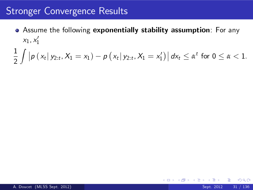
Stronger Convergence Results
Assume the following exponentially stability assumption: For any 0 x1 , x1 p ( xt j y2:t , X1 = x1 )
0 p xt j y2:t , X1 = x1
1 2
Z
dxt
t for 0
< 1.
A. Doucet (MLSS Sept. 2012)
Sept. 2012
31 / 136
104
![Slide: Stronger Convergence Results
Assume the following exponentially stability assumption: For any 0 x1 , x1 p ( xt j y2:t , X1 = x1 )
0 p xt j y2:t , X1 = x1
1 2
Z
dxt
t for 0
< 1.
Marginal distribution. For t (x1:t ) = (xt L:t ), there exists B1 , B2 < s.t. B1 c ( p ) k k 1/p p E [j b t t jp ] , N p lim N ( b t t ) ) N 0, 2 where 2 B2 , t t i.e. there is no accumulation of numerical errors over time.
N !
A. Doucet (MLSS Sept. 2012)
Sept. 2012
31 / 136](https://yosinski.com/mlss12/media/slides/MLSS-2012-Doucet-Sequential-Monte-Carlo-Methods_105.png)
Stronger Convergence Results
Assume the following exponentially stability assumption: For any 0 x1 , x1 p ( xt j y2:t , X1 = x1 )
0 p xt j y2:t , X1 = x1
1 2
Z
dxt
t for 0
< 1.
Marginal distribution. For t (x1:t ) = (xt L:t ), there exists B1 , B2 < s.t. B1 c ( p ) k k 1/p p E [j b t t jp ] , N p lim N ( b t t ) ) N 0, 2 where 2 B2 , t t i.e. there is no accumulation of numerical errors over time.
N !
A. Doucet (MLSS Sept. 2012)
Sept. 2012
31 / 136
105
![Slide: Stronger Convergence Results
Assume the following exponentially stability assumption: For any 0 x1 , x1 p ( xt j y2:t , X1 = x1 )
0 p xt j y2:t , X1 = x1
1 2
Z
dxt
t for 0
< 1.
i.e. there is no accumulation of numerical errors over time. b L1 distance. If p ( x1:t j y1:t ) = E (p ( x1:t j y1:t )), there exists B3 < s.t. Z B3 t ; jp ( x1:t j y1:t ) p ( x1:t j y1:t )j dx1:t N i.e. the bias only increases in t.
A. Doucet (MLSS Sept. 2012) Sept. 2012 31 / 136
Marginal distribution. For t (x1:t ) = (xt L:t ), there exists B1 , B2 < s.t. B1 c ( p ) k k 1/p p E [j b t t jp ] , N p lim N ( b t t ) ) N 0, 2 where 2 B2 , t t
N !](https://yosinski.com/mlss12/media/slides/MLSS-2012-Doucet-Sequential-Monte-Carlo-Methods_106.png)
Stronger Convergence Results
Assume the following exponentially stability assumption: For any 0 x1 , x1 p ( xt j y2:t , X1 = x1 )
0 p xt j y2:t , X1 = x1
1 2
Z
dxt
t for 0
< 1.
i.e. there is no accumulation of numerical errors over time. b L1 distance. If p ( x1:t j y1:t ) = E (p ( x1:t j y1:t )), there exists B3 < s.t. Z B3 t ; jp ( x1:t j y1:t ) p ( x1:t j y1:t )j dx1:t N i.e. the bias only increases in t.
A. Doucet (MLSS Sept. 2012) Sept. 2012 31 / 136
Marginal distribution. For t (x1:t ) = (xt L:t ), there exists B1 , B2 < s.t. B1 c ( p ) k k 1/p p E [j b t t jp ] , N p lim N ( b t t ) ) N 0, 2 where 2 B2 , t t
N !
106
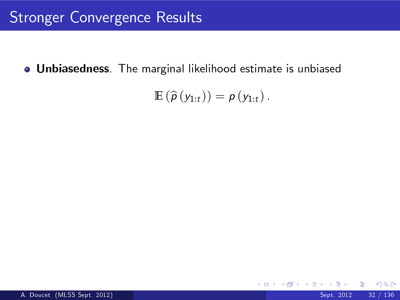
Stronger Convergence Results
Unbiasedness. The marginal likelihood estimate is unbiased E (p (y1:t )) = p (y1:t ) . b
A. Doucet (MLSS Sept. 2012)
Sept. 2012
32 / 136
107
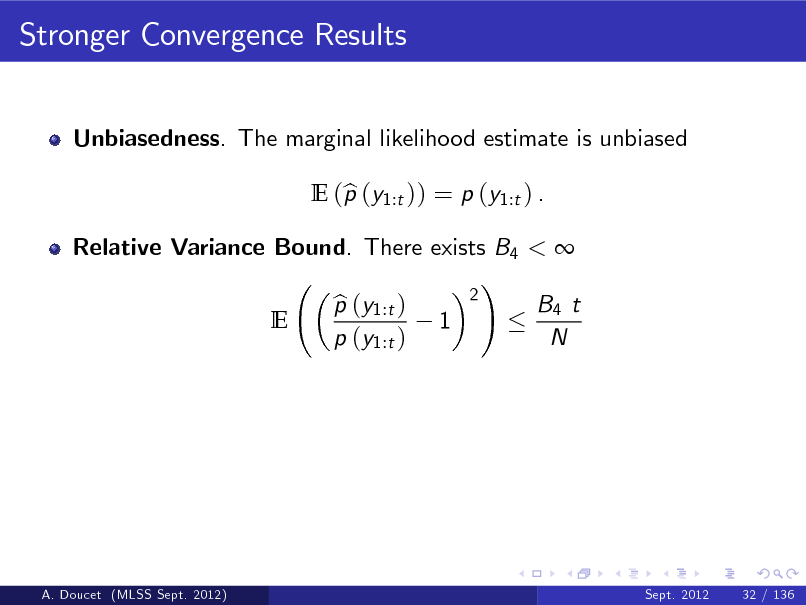
Stronger Convergence Results
Unbiasedness. The marginal likelihood estimate is unbiased E (p (y1:t )) = p (y1:t ) . b
Relative Variance Bound. There exists B4 < ! 2 p (y1:t ) b B4 t E 1 p (y1:t ) N
A. Doucet (MLSS Sept. 2012)
Sept. 2012
32 / 136
108
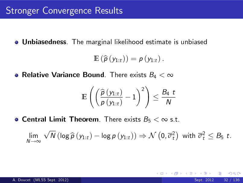
Stronger Convergence Results
Unbiasedness. The marginal likelihood estimate is unbiased E (p (y1:t )) = p (y1:t ) . b
Relative Variance Bound. There exists B4 < ! 2 p (y1:t ) b B4 t E 1 p (y1:t ) N
Central Limit Theorem. There exists B5 < s.t. p lim N (log p (y1:t ) log p (y1:t )) ) N 0, 2 with 2 b t t
N !
B5 t.
A. Doucet (MLSS Sept. 2012)
Sept. 2012
32 / 136
109
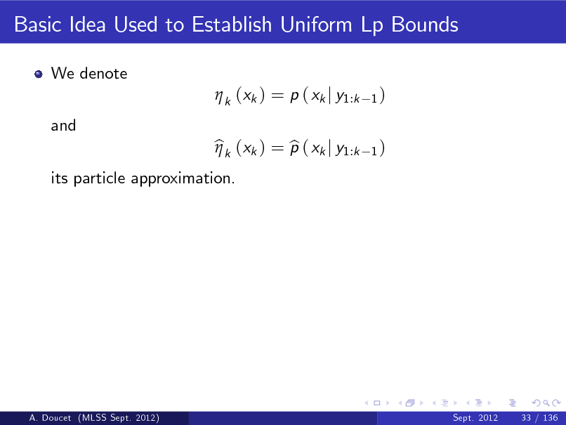
Basic Idea Used to Establish Uniform Lp Bounds
We denote k (xk ) = p ( xk j y1:k and its particle approximation. bk (xk ) = p ( xk j y1:k b
1) 1)
A. Doucet (MLSS Sept. 2012)
Sept. 2012
33 / 136
110
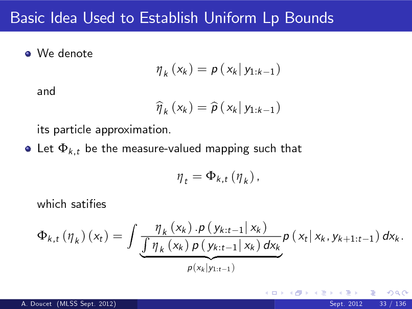
Basic Idea Used to Establish Uniform Lp Bounds
We denote k (xk ) = p ( xk j y1:k and its particle approximation. bk (xk ) = p ( xk j y1:k b t = k ,t ( k ) , which saties k ,t ( k ) (xt ) =
Z
1) 1)
Let k ,t be the measure-valued mapping such that
(x ) .p ( yk :t 1 j xk ) R k k p ( xt j xk , yk +1:t k (xk ) p ( yk :t 1 j xk ) dxk | {z }
p (xk jy1:t
1) Sept. 2012
1 ) dxk .
A. Doucet (MLSS Sept. 2012)
33 / 136
111
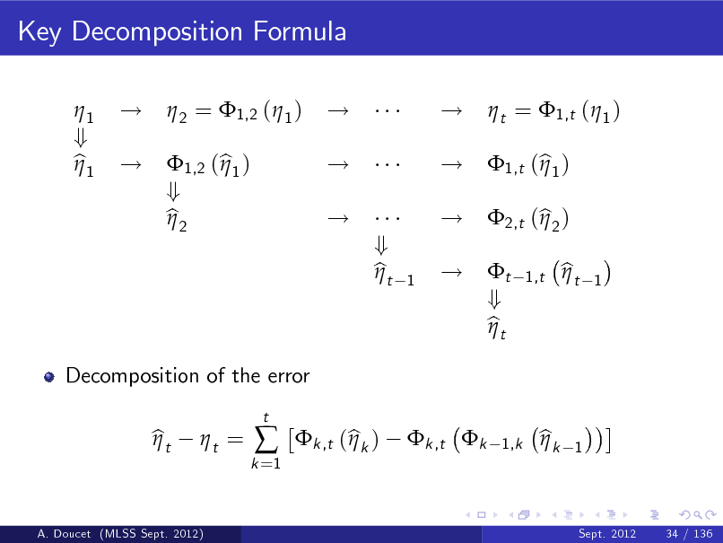
Key Decomposition Formula
1 + b1
! !
2 = 1,2 ( 1 ) 1,2 (b1 ) + b2
! ! ! + bt
! ! !
1
t = 1,t ( 1 ) 1,t (b1 )
1,t
!
Decomposition of the error bt t =
t + bt
2,t (b2 )
bt
1
k =1
t
k ,t (bk )
k ,t k
1,k
bk
1
A. Doucet (MLSS Sept. 2012)
Sept. 2012
34 / 136
112
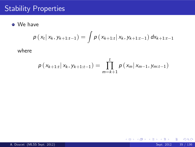
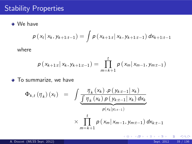
Stability Properties
We have p ( xt j xk , yk +1:t where p ( xk +1:t j xk , yk +1:t
1) 1) =
Z
p ( xk +1:t j xk , yk +1:t
t
1 ) dxk +1:t 1
=
m =k +1
p ( xm j xm
1 , ym:t 1 )
A. Doucet (MLSS Sept. 2012)
Sept. 2012
35 / 136
113
Stability Properties
We have p ( xt j xk , yk +1:t where p ( xk +1:t j xk , yk +1:t To summarize, we have k ,t ( k ) (xt ) =
Z
1) 1) =
Z
p ( xk +1:t j xk , yk +1:t
t
1 ) dxk +1:t 1
=
m =k +1
p ( xm j xm
1 , ym:t 1 )
(x ) .p ( yk :t 1 j xk ) R k k (xk ) p ( yk :t 1 j xk ) dxk | k {z }
m =k +1
t
p (xk jy1:t
1)
p ( xm j xm
1 , ym:t 1 ) dxk :t 1
A. Doucet (MLSS Sept. 2012)
Sept. 2012
35 / 136
114
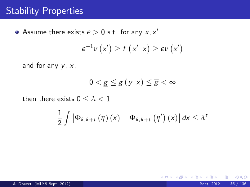
Stability Properties
Assume there exists
> 0 s.t. for any x, x 0
1
x0
f x0 x
x0
and for any y , x, 0<g then there exists 0 1 2
Z
g (yj x)
g <
<1 k ,k +t 0 (x ) dx t
k ,k +t ( ) (x )
A. Doucet (MLSS Sept. 2012)
Sept. 2012
36 / 136
115
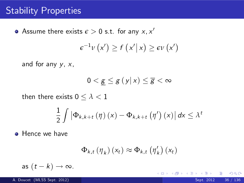
Stability Properties
Assume there exists
> 0 s.t. for any x, x 0
1
x0
f x0 x
x0
and for any y , x, 0<g then there exists 0 1 2
Z
g (yj x)
g <
<1 k ,k +t 0 (x ) dx t
k ,k +t ( ) (x )
Hence we have k ,t ( k ) (xt ) as (t k ) ! .
Sept. 2012 36 / 136
0 k ,t k (xt )
A. Doucet (MLSS Sept. 2012)
116

Putting Everything Together
Under such strong mixing assumptions bt t = |k ,t (bk )
t
k =1
1 ' p t N
k ,t k {z
k +1
1,k
for 0 1
bk
1
}
A. Doucet (MLSS Sept. 2012)
Sept. 2012
37 / 136
117
![Slide: Putting Everything Together
Under such strong mixing assumptions bt t = |k ,t (bk ) t jp ]
1/p t
k =1
1 ' p t N
We can then obtain results such as there exists B1 < s.t. E [j b t B1 c ( p ) k k p N
k ,t k {z
k +1
1,k
for 0 1
bk
1
}
A. Doucet (MLSS Sept. 2012)
Sept. 2012
37 / 136](https://yosinski.com/mlss12/media/slides/MLSS-2012-Doucet-Sequential-Monte-Carlo-Methods_118.png)
Putting Everything Together
Under such strong mixing assumptions bt t = |k ,t (bk ) t jp ]
1/p t
k =1
1 ' p t N
We can then obtain results such as there exists B1 < s.t. E [j b t B1 c ( p ) k k p N
k ,t k {z
k +1
1,k
for 0 1
bk
1
}
A. Doucet (MLSS Sept. 2012)
Sept. 2012
37 / 136
118
![Slide: Putting Everything Together
Under such strong mixing assumptions bt t = |k ,t (bk ) t jp ]
1/p t
k =1
1 ' p t N
We can then obtain results such as there exists B1 < s.t. E [j b t B1 c ( p ) k k p N
k ,t k {z
k +1
1,k
for 0 1
bk
1
}
Much work has been done recently on removing such strong mixing assumptions; e.g. Whiteley (2012) for much weaker and realistic assumptions.
A. Doucet (MLSS Sept. 2012)
Sept. 2012
37 / 136](https://yosinski.com/mlss12/media/slides/MLSS-2012-Doucet-Sequential-Monte-Carlo-Methods_119.png)
Putting Everything Together
Under such strong mixing assumptions bt t = |k ,t (bk ) t jp ]
1/p t
k =1
1 ' p t N
We can then obtain results such as there exists B1 < s.t. E [j b t B1 c ( p ) k k p N
k ,t k {z
k +1
1,k
for 0 1
bk
1
}
Much work has been done recently on removing such strong mixing assumptions; e.g. Whiteley (2012) for much weaker and realistic assumptions.
A. Doucet (MLSS Sept. 2012)
Sept. 2012
37 / 136
119
Summary
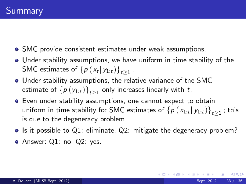
SMC provide consistent estimates under weak assumptions.
A. Doucet (MLSS Sept. 2012)
Sept. 2012
38 / 136
120
Summary
SMC provide consistent estimates under weak assumptions. Under stability assumptions, we have uniform in time stability of the SMC estimates of fp ( xt j y1:t )gt 1 .
A. Doucet (MLSS Sept. 2012)
Sept. 2012
38 / 136
121
Summary
SMC provide consistent estimates under weak assumptions. Under stability assumptions, we have uniform in time stability of the SMC estimates of fp ( xt j y1:t )gt 1 . Under stability assumptions, the relative variance of the SMC estimate of fp (y1:t )gt 1 only increases linearly with t.
A. Doucet (MLSS Sept. 2012)
Sept. 2012
38 / 136
122
Summary
SMC provide consistent estimates under weak assumptions. Under stability assumptions, we have uniform in time stability of the SMC estimates of fp ( xt j y1:t )gt 1 . Under stability assumptions, the relative variance of the SMC estimate of fp (y1:t )gt 1 only increases linearly with t.
Even under stability assumptions, one cannot expect to obtain uniform in time stability for SMC estimates of fp ( x1:t j y1:t )gt is due to the degeneracy problem.
1
; this
A. Doucet (MLSS Sept. 2012)
Sept. 2012
38 / 136
123
Summary
SMC provide consistent estimates under weak assumptions. Under stability assumptions, we have uniform in time stability of the SMC estimates of fp ( xt j y1:t )gt 1 . Under stability assumptions, the relative variance of the SMC estimate of fp (y1:t )gt 1 only increases linearly with t.
Even under stability assumptions, one cannot expect to obtain uniform in time stability for SMC estimates of fp ( x1:t j y1:t )gt is due to the degeneracy problem.
1
; this
Is it possible to Q1: eliminate, Q2: mitigate the degeneracy problem?
A. Doucet (MLSS Sept. 2012)
Sept. 2012
38 / 136
124
Summary
SMC provide consistent estimates under weak assumptions. Under stability assumptions, we have uniform in time stability of the SMC estimates of fp ( xt j y1:t )gt 1 . Under stability assumptions, the relative variance of the SMC estimate of fp (y1:t )gt 1 only increases linearly with t.
Even under stability assumptions, one cannot expect to obtain uniform in time stability for SMC estimates of fp ( x1:t j y1:t )gt is due to the degeneracy problem. Answer: Q1: no, Q2: yes.
1
; this
Is it possible to Q1: eliminate, Q2: mitigate the degeneracy problem?
A. Doucet (MLSS Sept. 2012)
Sept. 2012
38 / 136
125

Is Resampling Really Necessary?
Resampling is the source of the degeneracy problem and might appear wasteful.
A. Doucet (MLSS Sept. 2012)
Sept. 2012
39 / 136
126
![Slide: Is Resampling Really Necessary?
Resampling is the source of the degeneracy problem and might appear wasteful. The resampling step is an unbiased operation E [ p ( x1:t j y1:t )j p ( x1:t j y1:t )] = p ( x1:t j y1:t ) b e e V
Z
but clearly it introduces some errors locally in time. That is for any test function, we have V
Z
(x1:t ) p ( x1:t j y1:t ) dx1:t b
(x1:t ) p ( x1:t j y1:t ) dx1:t e
A. Doucet (MLSS Sept. 2012)
Sept. 2012
39 / 136](https://yosinski.com/mlss12/media/slides/MLSS-2012-Doucet-Sequential-Monte-Carlo-Methods_127.png)
Is Resampling Really Necessary?
Resampling is the source of the degeneracy problem and might appear wasteful. The resampling step is an unbiased operation E [ p ( x1:t j y1:t )j p ( x1:t j y1:t )] = p ( x1:t j y1:t ) b e e V
Z
but clearly it introduces some errors locally in time. That is for any test function, we have V
Z
(x1:t ) p ( x1:t j y1:t ) dx1:t b
(x1:t ) p ( x1:t j y1:t ) dx1:t e
A. Doucet (MLSS Sept. 2012)
Sept. 2012
39 / 136
127
![Slide: Is Resampling Really Necessary?
Resampling is the source of the degeneracy problem and might appear wasteful. The resampling step is an unbiased operation E [ p ( x1:t j y1:t )j p ( x1:t j y1:t )] = p ( x1:t j y1:t ) b e e V
Z
but clearly it introduces some errors locally in time. That is for any test function, we have V
Z
What about eliminating the resampling step?
(x1:t ) p ( x1:t j y1:t ) dx1:t b
(x1:t ) p ( x1:t j y1:t ) dx1:t e
A. Doucet (MLSS Sept. 2012)
Sept. 2012
39 / 136](https://yosinski.com/mlss12/media/slides/MLSS-2012-Doucet-Sequential-Monte-Carlo-Methods_128.png)
Is Resampling Really Necessary?
Resampling is the source of the degeneracy problem and might appear wasteful. The resampling step is an unbiased operation E [ p ( x1:t j y1:t )j p ( x1:t j y1:t )] = p ( x1:t j y1:t ) b e e V
Z
but clearly it introduces some errors locally in time. That is for any test function, we have V
Z
What about eliminating the resampling step?
(x1:t ) p ( x1:t j y1:t ) dx1:t b
(x1:t ) p ( x1:t j y1:t ) dx1:t e
A. Doucet (MLSS Sept. 2012)
Sept. 2012
39 / 136
128
Sequential Importance Samping: SMC Without Resampling
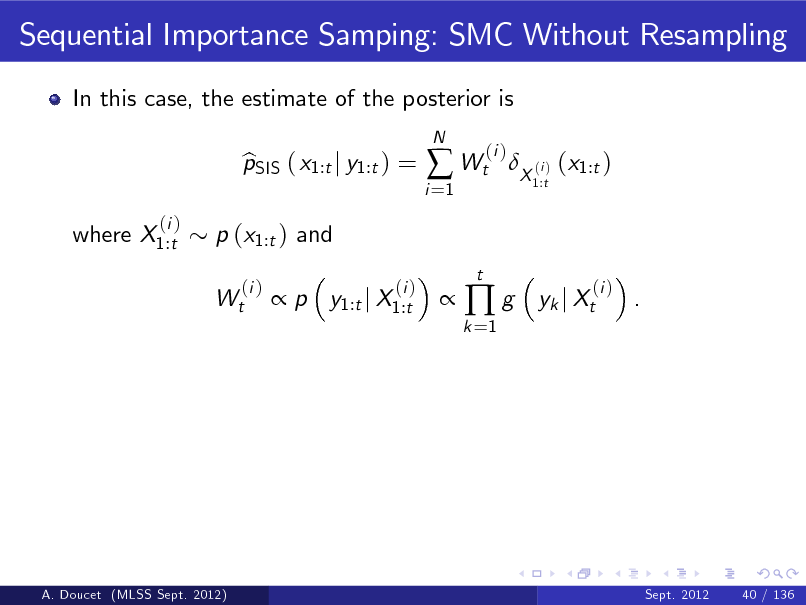
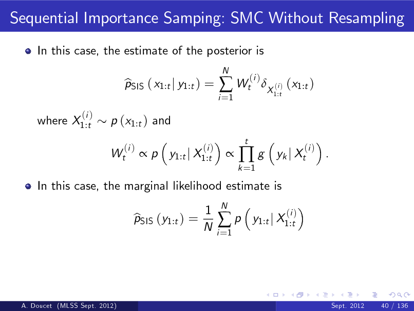
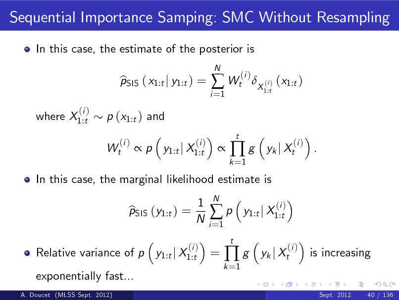
In this case, the estimate of the posterior is pSIS ( x1:t j y1:t ) = b p y1:t j X1:t
(i )
N
i =1
Wt
t
(i )
X (i ) (x1:t )
1:t
where X1:t
(i )
p (x1:t ) and Wt
(i )
k =1
g
yk j Xt
(i )
.
A. Doucet (MLSS Sept. 2012)
Sept. 2012
40 / 136
129
Sequential Importance Samping: SMC Without Resampling
In this case, the estimate of the posterior is pSIS ( x1:t j y1:t ) = b p y1:t j X1:t
(i )
N
i =1
Wt
t
(i )
X (i ) (x1:t )
1:t
where X1:t
(i )
p (x1:t ) and Wt
(i )
k =1
g
yk j Xt
(i )
.
In this case, the marginal likelihood estimate is pSIS (y1:t ) = b 1 N
i =1
p
N
y1:t j X1:t
(i )
A. Doucet (MLSS Sept. 2012)
Sept. 2012
40 / 136
130
Sequential Importance Samping: SMC Without Resampling
In this case, the estimate of the posterior is pSIS ( x1:t j y1:t ) = b p y1:t j X1:t
(i )
N
i =1
Wt
t
(i )
X (i ) (x1:t )
1:t
where X1:t
(i )
p (x1:t ) and Wt
(i )
k =1
g
yk j Xt
(i )
.
In this case, the marginal likelihood estimate is pSIS (y1:t ) = b 1 N
i =1
p
t
N
y1:t j X1:t
(i )
Relative variance of p y1:t j X1:t exponentially fast...
A. Doucet (MLSS Sept. 2012)
(i )
=
k =1
g
yk j Xt
(i )
is increasing
Sept. 2012
40 / 136
131
SIS For Stochastic Volatility Model
1000
500
0 - 25 1000
- 20
- 15
- 10
-5
0
500
0 - 25 100
- 20
- 15
- 10
-5
0
50
0 - 25
- 20
Importance Weights (base 10 logarithm)
- 15
- 10
-5
0
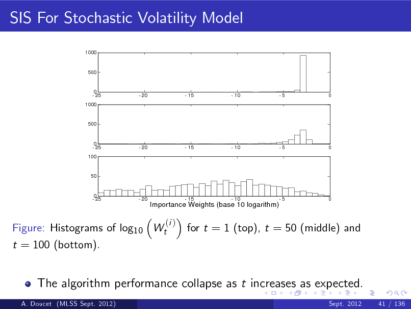
Figure: Histograms of log10 Wt t = 100 (bottom).
(i )
for t = 1 (top), t = 50 (middle) and
The algorithm performance collapse as t increases as expected.
A. Doucet (MLSS Sept. 2012) Sept. 2012 41 / 136
132
Central Limit Theorems
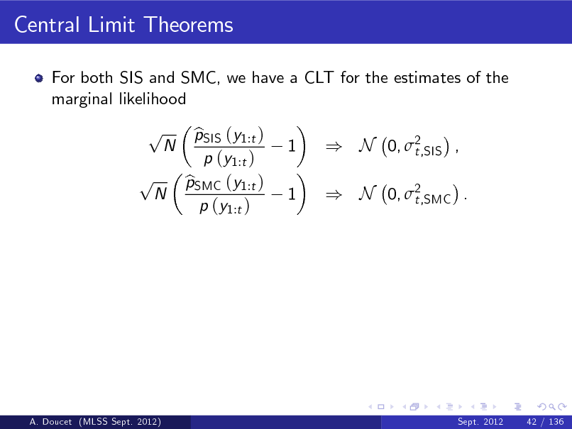
For both SIS and SMC, we have a CLT for the estimates of the marginal likelihood
p p
N
N
pSIS (y1:t ) b p (y1:t ) pSMC (y1:t ) b p (y1:t )
1 1
) N 0, 2 t,SIS , ) N 0, 2 t,SMC .
A. Doucet (MLSS Sept. 2012)
Sept. 2012
42 / 136
133

Central Limit Theorems
For both SIS and SMC, we have a CLT for the estimates of the marginal likelihood
p p
N
N
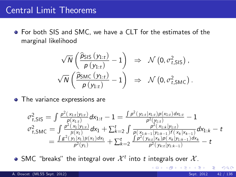
The variance expressions are 2 t,SIS =
pSIS (y1:t ) b p (y1:t ) pSMC (y1:t ) b p (y1:t )
1 1
) N 0, 2 t,SIS , ) N 0, 2 t,SMC .
2 t,SMC =
R
=
R 2 p ( y1:t jx1:t )p (x1:t )dx1:t p 2 ( x1:t jy1:t ) dx1:t 1 = 1 p (x1:t ) p 2 (y1:t ) R R p 2 ( x1 jy1:t ) 2( x p 1:k jy 1:t ) dx1 + t =2 p ( x dx1:k k R 2 (x 1 ) R 21:k 1 jy1:k 1 )f ( xk jxk 1 ) g ( y1 jx1 )(x1 )dx1 p ( yk :t jxk )p ( xk jy1:k 1 )dxk + t =2 t k p 2 (y 1 ) p 2 ( yk :t jy1:k 1 )
t
A. Doucet (MLSS Sept. 2012)
Sept. 2012
42 / 136
134
Central Limit Theorems
For both SIS and SMC, we have a CLT for the estimates of the marginal likelihood
p p
N
N
The variance expressions are 2 t,SIS =
pSIS (y1:t ) b p (y1:t ) pSMC (y1:t ) b p (y1:t )
1 1
) N 0, 2 t,SIS , ) N 0, 2 t,SMC .
2 t,SMC =
R
=
R 2 p ( y1:t jx1:t )p (x1:t )dx1:t p 2 ( x1:t jy1:t ) dx1:t 1 = 1 p (x1:t ) p 2 (y1:t ) R R p 2 ( x1 jy1:t ) 2( x p 1:k jy 1:t ) dx1 + t =2 p ( x dx1:k k R 2 (x 1 ) R 21:k 1 jy1:k 1 )f ( xk jxk 1 ) g ( y1 jx1 )(x1 )dx1 p ( yk :t jxk )p ( xk jy1:k 1 )dxk + t =2 t k p 2 (y 1 ) p 2 ( yk :t jy1:k 1 )
t
SMC breaks the integral over X t into t integrals over X .
A. Doucet (MLSS Sept. 2012) Sept. 2012 42 / 136
135
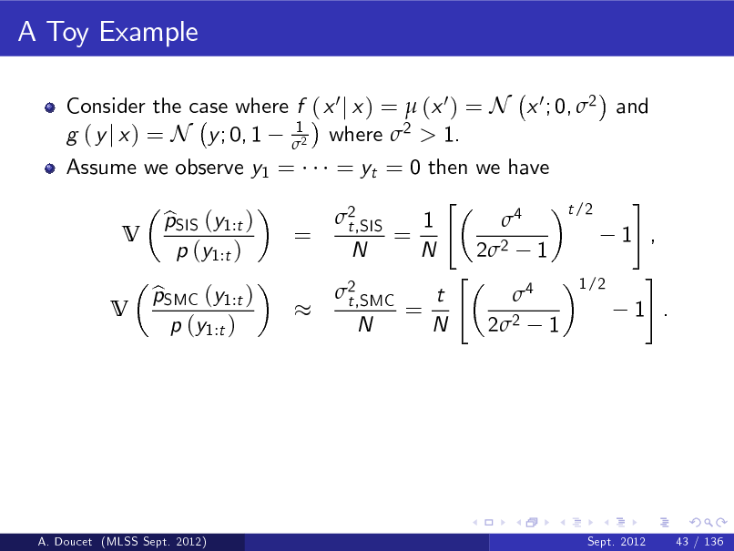
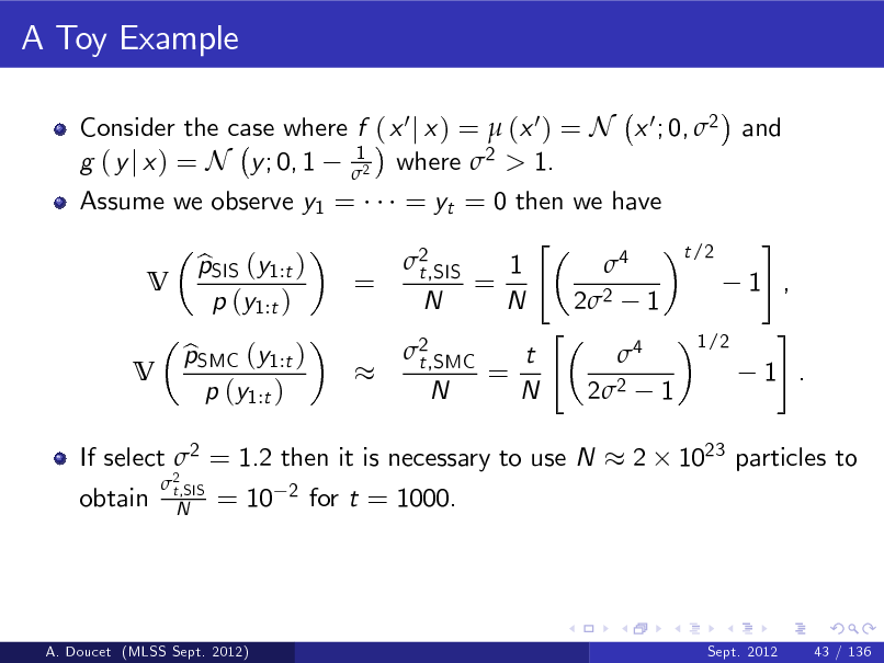
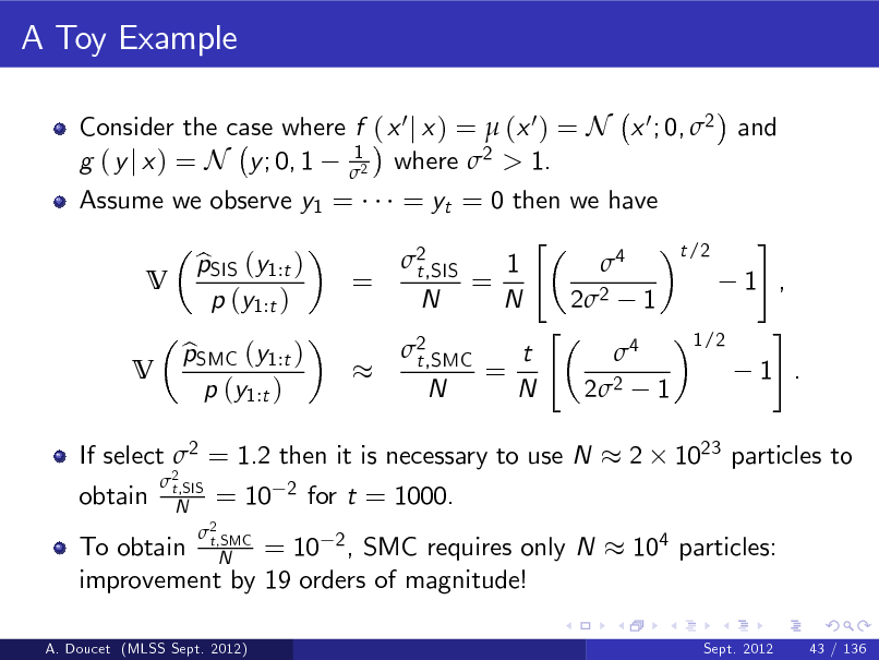
A Toy Example
Consider the case where f ( x 0 j x ) = (x 0 ) = N x 0 ; 0, 2 and 1 g ( y j x ) = N y ; 0, 1 2 where 2 > 1.
A. Doucet (MLSS Sept. 2012)
Sept. 2012
43 / 136
136
A Toy Example
Consider the case where f ( x 0 j x ) = (x 0 ) = N x 0 ; 0, 2 and 1 g ( y j x ) = N y ; 0, 1 2 where 2 > 1. Assume we observe y1 = V V pSIS (y1:t ) b p (y1:t )
=
pSMC (y1:t ) b p (y1:t )
= yt = 0 then we have " 2 1 4 t,SIS = N N 22 1 " 2 t 4 t,SMC = N N 22 1
t /2
1 ,
1/2
#
1 .
#
A. Doucet (MLSS Sept. 2012)
Sept. 2012
43 / 136
137
A Toy Example
Consider the case where f ( x 0 j x ) = (x 0 ) = N x 0 ; 0, 2 and 1 g ( y j x ) = N y ; 0, 1 2 where 2 > 1. Assume we observe y1 = V V pSIS (y1:t ) b p (y1:t )
=
pSMC (y1:t ) b p (y1:t )
2 t,SIS N
= yt = 0 then we have " 2 1 4 t,SIS = N N 22 1 " 2 t 4 t,SMC = N N 22 1
2
t /2
1 ,
1/2
#
1 . 1023 particles to
#
If select 2 = 1.2 then it is necessary to use N obtain
= 10
2
for t = 1000.
A. Doucet (MLSS Sept. 2012)
Sept. 2012
43 / 136
138
A Toy Example
Consider the case where f ( x 0 j x ) = (x 0 ) = N x 0 ; 0, 2 and 1 g ( y j x ) = N y ; 0, 1 2 where 2 > 1. Assume we observe y1 = V V pSIS (y1:t ) b p (y1:t )
=
pSMC (y1:t ) b p (y1:t )
2 t,SIS N
= yt = 0 then we have " 2 1 4 t,SIS = N N 22 1 " 2 t 4 t,SMC = N N 22 1
2
t /2
1 ,
1/2
#
1 . 1023 particles to
#
If select 2 = 1.2 then it is necessary to use N obtain
= 10
2
for t = 1000. 104 particles:
To obtain N = 10 2 , SMC requires only N improvement by 19 orders of magnitude!
A. Doucet (MLSS Sept. 2012)
2 t,SMC
Sept. 2012
43 / 136
139
Better Resampling Schemes
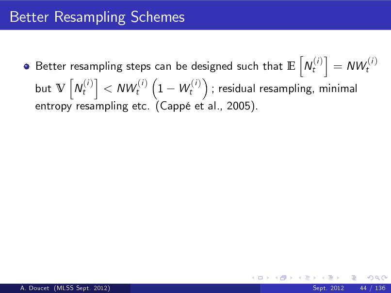
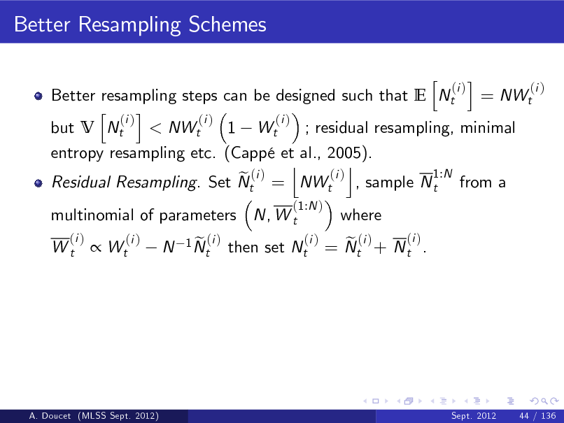
h i (i ) (i ) Better resampling steps can be designed such that E Nt = NWt h i (i ) (i ) (i ) but V Nt < NWt 1 Wt ; residual resampling, minimal entropy resampling etc. (Capp et al., 2005).
A. Doucet (MLSS Sept. 2012)
Sept. 2012
44 / 136
140
Better Resampling Schemes
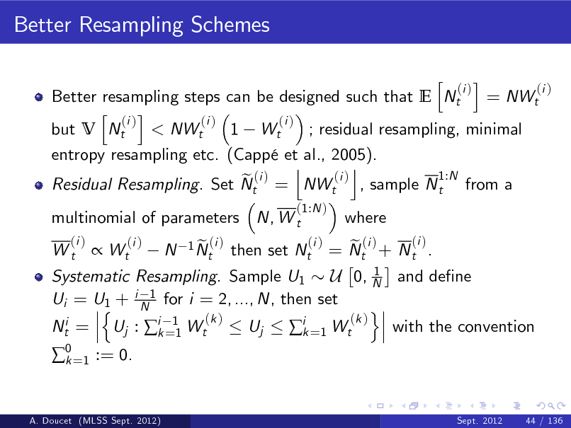
h i (i ) (i ) Better resampling steps can be designed such that E Nt = NWt h i (i ) (i ) (i ) but V Nt < NWt 1 Wt ; residual resampling, minimal entropy resampling etc. (Capp et al., 2005). j k 1:N (i ) e (i ) Residual Resampling. Set Nt = NWt , sample N t from a
(1:N ) (i )
multinomial of parameters N, W t
(i ) Wt
where
Wt
(i )
N
1 N (i ) et
then set Nt
(i ) e (i ) = Nt + N t .
A. Doucet (MLSS Sept. 2012)
Sept. 2012
44 / 136
141
Better Resampling Schemes
h i (i ) (i ) Better resampling steps can be designed such that E Nt = NWt h i (i ) (i ) (i ) but V Nt < NWt 1 Wt ; residual resampling, minimal entropy resampling etc. (Capp et al., 2005). j k 1:N (i ) e (i ) Residual Resampling. Set Nt = NWt , sample N t from a
(1:N ) (i )
multinomial of parameters N, W t
(i ) Wt
where
(i ) e (i ) = Nt + N t . 1 Systematic Resampling. Sample U1 U 0, N and dene Ui = U1 + i N1 for i = 2, ..., N, then set n o (k ) (k ) Nti = Uj : ik =11 Wt Uj with the convention ik =1 Wt
Wt
(i )
N
1 N (i ) et
then set Nt
0 =1 := 0. k
A. Doucet (MLSS Sept. 2012)
Sept. 2012
44 / 136
142

Measuring Variability of the Weights
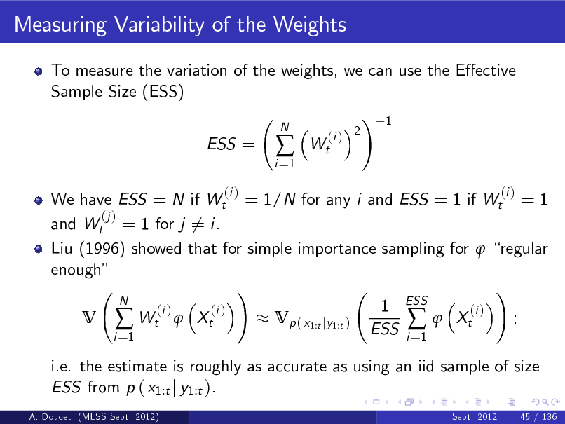
To measure the variation of the weights, we can use the Eective Sample Size (ESS) ! 1 ESS =
i =1
N
Wt
(i ) 2
A. Doucet (MLSS Sept. 2012)
Sept. 2012
45 / 136
143

Measuring Variability of the Weights
To measure the variation of the weights, we can use the Eective Sample Size (ESS) ! 1 ESS =
(i )
i =1
N
Wt
(i ) 2
We have ESS = N if Wt (j ) and Wt = 1 for j 6= i.
= 1/N for any i and ESS = 1 if Wt
(i )
=1
A. Doucet (MLSS Sept. 2012)
Sept. 2012
45 / 136
144
Measuring Variability of the Weights
To measure the variation of the weights, we can use the Eective Sample Size (ESS) ! 1 ESS =
(i )
i =1
N
Wt
(i ) 2
We have ESS = N if Wt = 1/N for any i and ESS = 1 if Wt = 1 (j ) and Wt = 1 for j 6= i. Liu (1996) showed that for simple importance sampling for regular enough ! ! N 1 ESS (i ) (i ) (i ) V Wt Xt Vp ( x1:t jy1:t ) Xt ; ESS i i =1 =1 i.e. the estimate is roughly as accurate as using an iid sample of size ESS from p ( x1:t j y1:t ).
A. Doucet (MLSS Sept. 2012) Sept. 2012 45 / 136
(i )
145
Dynamic Resampling
Resampling at each time step can be harmful: only resample when necessary.
A. Doucet (MLSS Sept. 2012)
Sept. 2012
46 / 136
146
Dynamic Resampling
Resampling at each time step can be harmful: only resample when necessary. Dynamic Resampling: If the variation of the weights as measured by ESS is too high, e.g. ESS < N/2, then resample the particles.
A. Doucet (MLSS Sept. 2012)
Sept. 2012
46 / 136
147
Dynamic Resampling
Resampling at each time step can be harmful: only resample when necessary. Dynamic Resampling: If the variation of the weights as measured by ESS is too high, e.g. ESS < N/2, then resample the particles. We can also use the entropy Ent =
i =1
Wt
N
(i )
log2 Wt
(i )
A. Doucet (MLSS Sept. 2012)
Sept. 2012
46 / 136
148
Dynamic Resampling
Resampling at each time step can be harmful: only resample when necessary. Dynamic Resampling: If the variation of the weights as measured by ESS is too high, e.g. ESS < N/2, then resample the particles. We can also use the entropy Ent =
i =1
Wt
(i )
N
(i )
log2 Wt
(i )
We have Ent = log2 (N ) if Wt = 1/N for any i. We have Ent = 0 (i ) (j ) if Wt = 1 and Wt = 1 for j 6= i.
A. Doucet (MLSS Sept. 2012)
Sept. 2012
46 / 136
149
Improving the Sampling Step
Bootstrap lter. Sample particles blindly according to the prior without taking into account the observation Very ine cient for vague prior/peaky likelihood.
A. Doucet (MLSS Sept. 2012)
Sept. 2012
47 / 136
150
Improving the Sampling Step
Bootstrap lter. Sample particles blindly according to the prior without taking into account the observation Very ine cient for vague prior/peaky likelihood. Optimal proposal/Perfect adaptation. Implement the following alternative update-propagate Bayesian recursion Update Propagate where p ( xt j yt , xt
1)
tj t 1 1:t 1 j 1:t 1 p ( x1:t 1 j y1:t ) = p ( yt jy1:t 1 ) p ( x1:t j y1:t ) = p ( x1:t 1 j y1:t ) p ( xt j yt , xt
p( y x
)p ( x
y
)
1)
=
Much more e cient when applicable; e.g. f ( xt j xt 1 ) = N (xt ; (xt 1 ) , v ) , g ( yt j xt ) = N (yt ; xt , w ) .
A. Doucet (MLSS Sept. 2012) Sept. 2012 47 / 136
f ( xt j xt 1 ) g ( yt j xt p ( yt j xt 1 )
1)
151
A General Bayesian Recursion
Introduce an arbitrary proposal distribution q ( xt j yt , xt approximation to p ( xt j yt , xt 1 ) .
1 );
i.e. an
A. Doucet (MLSS Sept. 2012)
Sept. 2012
48 / 136
152
A General Bayesian Recursion
Introduce an arbitrary proposal distribution q ( xt j yt , xt approximation to p ( xt j yt , xt 1 ) . We have seen that p ( x1:t j y1:t ) = so clearly p ( x1:t j y1:t ) = where w (xt
1 , xt , yt ) 1 );
i.e. an
g ( yt j xt ) f ( xt j xt 1 ) p ( x1:t p ( yt j y1:t 1 )
1 , xt , yt ) q
1 j y1:t 1 )
w (xt
( xt j yt , xt p ( yt j y1:t
1 ) p ( x1:t 1 j y1:t 1 ) 1)
=
g ( yt j xt ) f ( xt j xt q ( xt j yt , xt 1 )
1)
A. Doucet (MLSS Sept. 2012)
Sept. 2012
48 / 136
153
A General Bayesian Recursion
Introduce an arbitrary proposal distribution q ( xt j yt , xt approximation to p ( xt j yt , xt 1 ) . We have seen that p ( x1:t j y1:t ) = so clearly p ( x1:t j y1:t ) = where w (xt
1 , xt , yt ) 1 );
i.e. an
g ( yt j xt ) f ( xt j xt 1 ) p ( x1:t p ( yt j y1:t 1 )
1 , xt , yt ) q
1 j y1:t 1 )
w (xt
( xt j yt , xt p ( yt j y1:t
1 ) p ( x1:t 1 j y1:t 1 ) 1)
=
This suggests a more general SMC algorithm.
A. Doucet (MLSS Sept. 2012)
g ( yt j xt ) f ( xt j xt q ( xt j yt , xt 1 )
1)
Sept. 2012
48 / 136
154
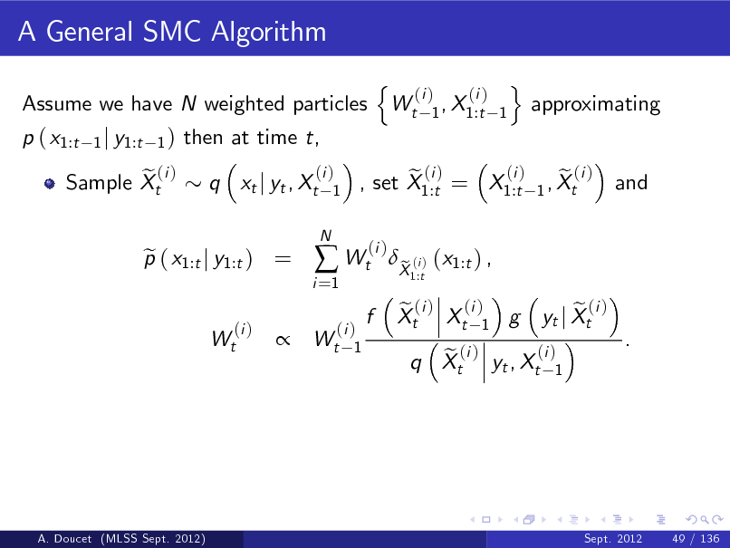
A General SMC Algorithm
Assume we have N weighted particles p ( x1:t e (i ) Sample Xt
1 j y1:t 1 )
then at time t, q xt j yt , Xt
(i ) 1
N
n
Wt
(i ) (i ) 1 , X1:t 1
o
approximating
p ( x1:t j y1:t ) = e
(i ) Wt
i =1
Wt
(i ) e (i ) e (i ) , set X1:t = X1:t 1 , Xt (i )
and
(i ) Wt 1
f
X (i ) (x1:t ) , e
1:t
e (i ) (i ) Xt Xt 1 g
(i ) e (i ) q Xt yt , Xt 1
e (i ) yt j Xt
.
A. Doucet (MLSS Sept. 2012)
Sept. 2012
49 / 136
155
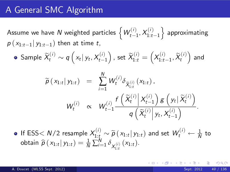
A General SMC Algorithm
Assume we have N weighted particles p ( x1:t e (i ) Sample Xt
1 j y1:t 1 )
then at time t, q xt j yt , Xt
(i ) 1
N
n
Wt
(i ) (i ) 1 , X1:t 1
o
approximating
p ( x1:t j y1:t ) = e
(i ) Wt
i =1
Wt
(i ) e (i ) e (i ) , set X1:t = X1:t 1 , Xt (i )
and
(i ) Wt 1
f
X (i ) (x1:t ) , e
1:t
e (i ) (i ) Xt Xt 1 g
If ESS< N/2 resample X1:t p ( x1:t j y1:t ) and set Wt e N 1 obtain p ( x1:t j y1:t ) = N i =1 X (i ) (x1:t ). b
1:t A. Doucet (MLSS Sept. 2012)
(i )
(i ) e (i ) q Xt yt , Xt 1
e (i ) yt j Xt
(i )
.
1 N
to
Sept. 2012
49 / 136
156

Building Proposals
Our aim is to select q ( xt j yt , xt 1 ) as close as possible to p ( xt j yt , xt 1 ) as this minimizes the variance of w (xt
1 , xt , yt )
=
g ( yt j xt ) f ( xt j xt q ( xt j yt , xt 1 )
1)
.
A. Doucet (MLSS Sept. 2012)
Sept. 2012
50 / 136
157

Building Proposals
Our aim is to select q ( xt j yt , xt 1 ) as close as possible to p ( xt j yt , xt 1 ) as this minimizes the variance of w (xt
1 , xt , yt )
=
Example - EKF proposal: Let Xt = ( Xt with Vt Yt
g ( yt j xt ) f ( xt j xt q ( xt j yt , xt 1 )
1)
.
1 ) + Vt ,
Yt = (Xt ) + Wt ,
N (0, v ), Wt
( (Xt
1 )) +
(x ) x
N (0, w ). We perform local linearization ( Xt
(X t
1)
( Xt
1 )) + Wt
and use as a proposal. q ( xt j yt , xt
1)
g ( yt j xt ) f ( xt j xt b
1) .
A. Doucet (MLSS Sept. 2012)
Sept. 2012
50 / 136
158
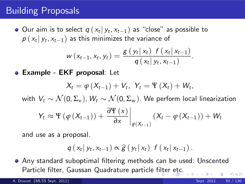
Building Proposals
Our aim is to select q ( xt j yt , xt 1 ) as close as possible to p ( xt j yt , xt 1 ) as this minimizes the variance of w (xt
1 , xt , yt )
=
Example - EKF proposal: Let Xt = ( Xt with Vt Yt
g ( yt j xt ) f ( xt j xt q ( xt j yt , xt 1 )
1)
.
1 ) + Vt ,
Yt = (Xt ) + Wt ,
N (0, v ), Wt
( (Xt
1 )) +
(x ) x
N (0, w ). We perform local linearization ( Xt
(X t
1)
( Xt
1 )) + Wt
and use as a proposal. q ( xt j yt , xt
1)
Any standard suboptimal ltering methods can be used: Unscented Particle lter, Gaussan Quadrature particle lter etc.
A. Doucet (MLSS Sept. 2012) Sept. 2012 50 / 136
g ( yt j xt ) f ( xt j xt b
1) .
159
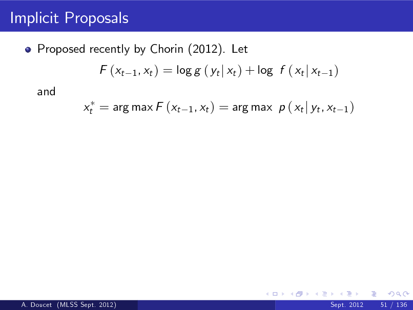
Implicit Proposals
Proposed recently by Chorin (2012). Let F (xt and
1 , xt )
= log g ( yt j xt ) + log f ( xt j xt
1 , xt )
1)
xt = arg max F (xt
= arg max p ( xt j yt , xt
1)
A. Doucet (MLSS Sept. 2012)
Sept. 2012
51 / 136
160
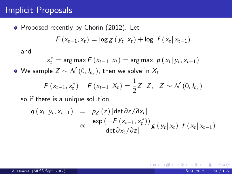
Implicit Proposals
Proposed recently by Chorin (2012). Let F (xt and
1 , xt )
= log g ( yt j xt ) + log f ( xt j xt
1 , xt )
1)
= arg max p ( xt j yt , xt 1 ) We sample Z N (0, Inx ), then we solve in Xt 1 F (xt 1 , xt ) F (xt 1 , Xt ) = Z T Z , Z N (0, Inx ) 2 so if there is a unique solution
q ( xt j yt , xt
1)
xt = arg max F (xt
= pZ (z ) jdet z/xt j exp ( F (xt 1 , xt )) g ( yt j xt ) f ( xt j xt jdet xt /z j
1)
A. Doucet (MLSS Sept. 2012)
Sept. 2012
51 / 136
161
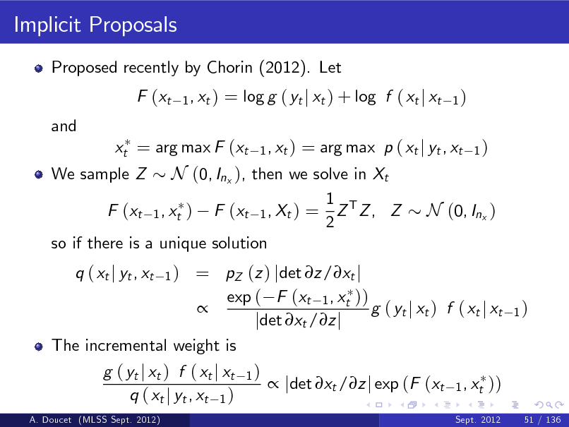
Implicit Proposals
Proposed recently by Chorin (2012). Let F (xt and
1 , xt )
= log g ( yt j xt ) + log f ( xt j xt
1 , xt )
1)
= arg max p ( xt j yt , xt 1 ) We sample Z N (0, Inx ), then we solve in Xt 1 F (xt 1 , xt ) F (xt 1 , Xt ) = Z T Z , Z N (0, Inx ) 2 so if there is a unique solution = pZ (z ) jdet z/xt j exp ( F (xt 1 , xt )) g ( yt j xt ) f ( xt j xt jdet xt /z j The incremental weight is g ( yt j xt ) f ( xt j xt 1 ) jdet xt /z j exp (F (xt 1 , xt )) q ( xt j yt , xt 1 )
q ( xt j yt , xt
1)
Sept. 2012
xt = arg max F (xt
1)
A. Doucet (MLSS Sept. 2012)
51 / 136
162

Auxiliary Particle Filters
Popular variation introduced by (Pitt & Shephard, 1999).
A. Doucet (MLSS Sept. 2012)
Sept. 2012
52 / 136
163
Auxiliary Particle Filters
Popular variation introduced by (Pitt & Shephard, 1999). This corresponds to a standard SMC algorithm (Johansen & D., 2008) where we target p ( x1:t j y1:t +1 ) p ( x1:t j y1:t ) p ( yt +1 j xt ) b b
where p ( yt +1 j xt ) b
b p ( yt +1 j xt ) using a proposal p ( xt j yt , xt
1 ).
A. Doucet (MLSS Sept. 2012)
Sept. 2012
52 / 136
164
Auxiliary Particle Filters
Popular variation introduced by (Pitt & Shephard, 1999). This corresponds to a standard SMC algorithm (Johansen & D., 2008) where we target p ( x1:t j y1:t +1 ) p ( x1:t j y1:t ) p ( yt +1 j xt ) b b
When p ( yt +1 j xt ) = p ( yt +1 j xt ) and b p ( xt +1 j yt +1 , xt ) = p ( xt +1 j yt +1 , xt ) then we are back to perfect b adaptation.
where p ( yt +1 j xt ) b
b p ( yt +1 j xt ) using a proposal p ( xt j yt , xt
1 ).
A. Doucet (MLSS Sept. 2012)
Sept. 2012
52 / 136
165
![Slide: Block Sampling Proposals
Problem: we only sample Xt at time t so, even if you use p ( xt j yt , xt 1 ), the SMC estimates could have high variance if Vp ( xt 1 jy1:t 1 ) [p ( yt j xt 1 )] is high.
A. Doucet (MLSS Sept. 2012)
Sept. 2012
53 / 136](https://yosinski.com/mlss12/media/slides/MLSS-2012-Doucet-Sequential-Monte-Carlo-Methods_166.png)
Block Sampling Proposals
Problem: we only sample Xt at time t so, even if you use p ( xt j yt , xt 1 ), the SMC estimates could have high variance if Vp ( xt 1 jy1:t 1 ) [p ( yt j xt 1 )] is high.
A. Doucet (MLSS Sept. 2012)
Sept. 2012
53 / 136
166
![Slide: Block Sampling Proposals
Problem: we only sample Xt at time t so, even if you use p ( xt j yt , xt 1 ), the SMC estimates could have high variance if Vp ( xt 1 jy1:t 1 ) [p ( yt j xt 1 )] is high. Block sampling idea: allows yourself to sample again Xt L +1:t 1 as well as Xt in light of yt . Optimally we would like at time t to sample Xt and
(i ) Wt (i ) L +1:t
p xt
(i ) L +1:t j yt L +1:t , Xt L
(i ) Wt 1
p X1:t y1:t p X1:t
(i )
L
(i )
y1:t
1
p Xt
(i ) L +1:t
yt
(i ) L +1:t , Xt L
Wt
(i ) 1p
yt j yt
(i ) L +1:t 1 , Xt L
A. Doucet (MLSS Sept. 2012)
Sept. 2012
53 / 136](https://yosinski.com/mlss12/media/slides/MLSS-2012-Doucet-Sequential-Monte-Carlo-Methods_167.png)
Block Sampling Proposals
Problem: we only sample Xt at time t so, even if you use p ( xt j yt , xt 1 ), the SMC estimates could have high variance if Vp ( xt 1 jy1:t 1 ) [p ( yt j xt 1 )] is high. Block sampling idea: allows yourself to sample again Xt L +1:t 1 as well as Xt in light of yt . Optimally we would like at time t to sample Xt and
(i ) Wt (i ) L +1:t
p xt
(i ) L +1:t j yt L +1:t , Xt L
(i ) Wt 1
p X1:t y1:t p X1:t
(i )
L
(i )
y1:t
1
p Xt
(i ) L +1:t
yt
(i ) L +1:t , Xt L
Wt
(i ) 1p
yt j yt
(i ) L +1:t 1 , Xt L
A. Doucet (MLSS Sept. 2012)
Sept. 2012
53 / 136
167
![Slide: Block Sampling Proposals
Problem: we only sample Xt at time t so, even if you use p ( xt j yt , xt 1 ), the SMC estimates could have high variance if Vp ( xt 1 jy1:t 1 ) [p ( yt j xt 1 )] is high. Block sampling idea: allows yourself to sample again Xt L +1:t 1 as well as Xt in light of yt . Optimally we would like at time t to sample Xt and
(i ) Wt (i ) L +1:t
p xt
(i ) L +1:t j yt L +1:t , Xt L
(i ) Wt 1
p X1:t y1:t p X1:t
(i )
L
(i )
y1:t
1
p Xt
(i ) L +1:t
yt
(i ) L +1:t , Xt L
Wt
(i ) 1p
yt j yt
(i ) L +1:t 1 , Xt L
When p ( xt L +1:t j yt L +1:t , xt L ) and p ( yt j yt L +1:t 1 , xt L ) are not available, we can use analytical approximations of them and still have consistent estimates (D., Briers & Senecal, 2006).
A. Doucet (MLSS Sept. 2012) Sept. 2012 53 / 136](https://yosinski.com/mlss12/media/slides/MLSS-2012-Doucet-Sequential-Monte-Carlo-Methods_168.png)
Block Sampling Proposals
Problem: we only sample Xt at time t so, even if you use p ( xt j yt , xt 1 ), the SMC estimates could have high variance if Vp ( xt 1 jy1:t 1 ) [p ( yt j xt 1 )] is high. Block sampling idea: allows yourself to sample again Xt L +1:t 1 as well as Xt in light of yt . Optimally we would like at time t to sample Xt and
(i ) Wt (i ) L +1:t
p xt
(i ) L +1:t j yt L +1:t , Xt L
(i ) Wt 1
p X1:t y1:t p X1:t
(i )
L
(i )
y1:t
1
p Xt
(i ) L +1:t
yt
(i ) L +1:t , Xt L
Wt
(i ) 1p
yt j yt
(i ) L +1:t 1 , Xt L
When p ( xt L +1:t j yt L +1:t , xt L ) and p ( yt j yt L +1:t 1 , xt L ) are not available, we can use analytical approximations of them and still have consistent estimates (D., Briers & Senecal, 2006).
A. Doucet (MLSS Sept. 2012) Sept. 2012 53 / 136
168

Block Sampling Proposals
Computational cost is increased from O (N ) to O (LN ) so is it worth it?
A. Doucet (MLSS Sept. 2012)
Sept. 2012
54 / 136
169
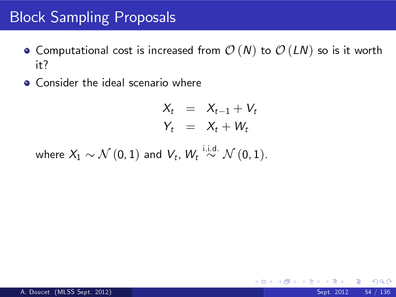
Block Sampling Proposals
Computational cost is increased from O (N ) to O (LN ) so is it worth it? Consider the ideal scenario where Xt Yt where X1
= Xt 1 + Vt = Xt + W t
i.i.d.
N (0, 1) and Vt , Wt
N (0, 1).
A. Doucet (MLSS Sept. 2012)
Sept. 2012
54 / 136
170
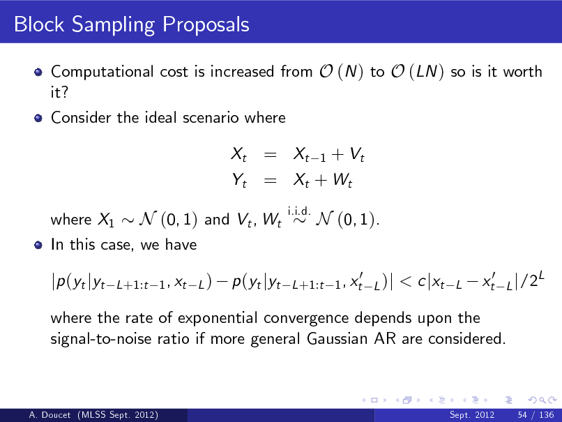
Block Sampling Proposals
Computational cost is increased from O (N ) to O (LN ) so is it worth it? Consider the ideal scenario where Xt Yt
= Xt 1 + Vt = Xt + W t
i.i.d.
where X1 N (0, 1) and Vt , Wt In this case, we have
N (0, 1). < c jxt
L
jp (yt jyt
L +1:t 1 , xt L )
p (yt jyt
0 L +1:t 1 , xt L )j
xt0
L j /2
L
where the rate of exponential convergence depends upon the signal-to-noise ratio if more general Gaussian AR are considered.
A. Doucet (MLSS Sept. 2012)
Sept. 2012
54 / 136
171
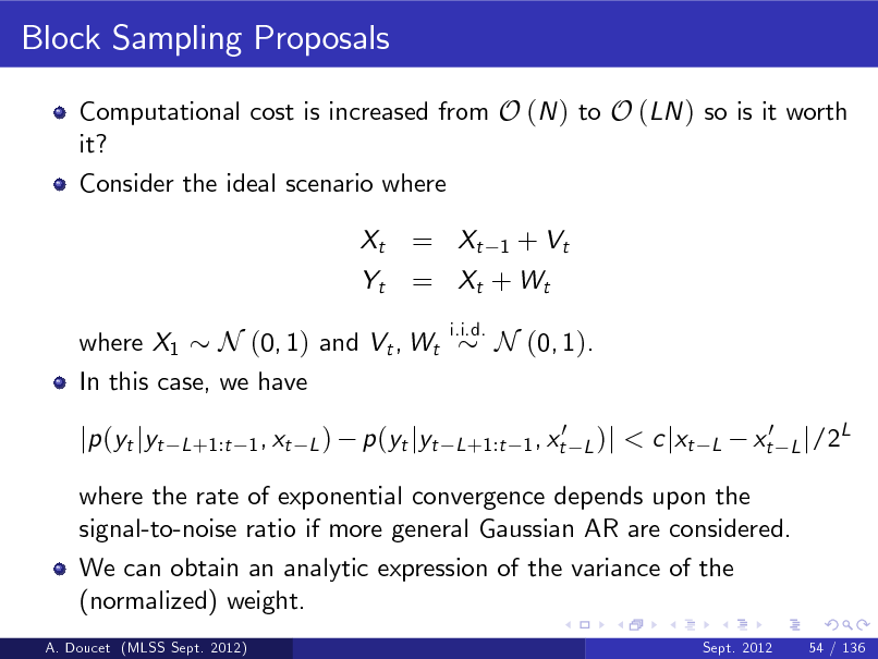
Block Sampling Proposals
Computational cost is increased from O (N ) to O (LN ) so is it worth it? Consider the ideal scenario where Xt Yt
= Xt 1 + Vt = Xt + W t
i.i.d.
where X1 N (0, 1) and Vt , Wt In this case, we have
N (0, 1). < c jxt
L
jp (yt jyt
L +1:t 1 , xt L )
p (yt jyt
0 L +1:t 1 , xt L )j
xt0
L j /2
L
where the rate of exponential convergence depends upon the signal-to-noise ratio if more general Gaussian AR are considered. We can obtain an analytic expression of the variance of the (normalized) weight.
A. Doucet (MLSS Sept. 2012) Sept. 2012 54 / 136
172
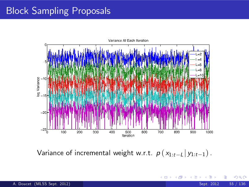
Block Sampling Proposals
Variance of incremental weight w.r.t. p ( x1:t
L j y1:t 1 ) .
A. Doucet (MLSS Sept. 2012)
Sept. 2012
55 / 136
173
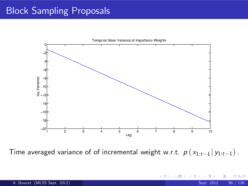
Block Sampling Proposals
Time averaged variance of of incremental weight w.r.t. p ( x1:t
L j y1:t 1 ) .
A. Doucet (MLSS Sept. 2012)
Sept. 2012
56 / 136
174

Fighting Degeneracy Using MCMC Steps
The design of good proposals can be complicated and/or time consuming so, after the resampling step, a few particles might inherit many ospring.
A. Doucet (MLSS Sept. 2012)
Sept. 2012
57 / 136
175

Fighting Degeneracy Using MCMC Steps
The design of good proposals can be complicated and/or time consuming so, after the resampling step, a few particles might inherit many ospring. A standard way to limit degeneracy is known as the Resample-Move algorithm (Gilks & Berzuini, 2001); i.e. using MCMC kernels as a principled way to jitter the particle locations.
A. Doucet (MLSS Sept. 2012)
Sept. 2012
57 / 136
176

Fighting Degeneracy Using MCMC Steps
The design of good proposals can be complicated and/or time consuming so, after the resampling step, a few particles might inherit many ospring. A standard way to limit degeneracy is known as the Resample-Move algorithm (Gilks & Berzuini, 2001); i.e. using MCMC kernels as a principled way to jitter the particle locations.
0 A MCMC kernel Kt ( x1:t j x1:t ) of invariant distribution p ( x1:t j y1:t ) is a Markov transition kernel with the property that 0 p x1:t y1:t =
Z
0 p ( x1:t j y1:t ) Kt x1:t x1:t dx1:t , 0 Kt ( x1:t j X1:t ) then
0 i.e. if X1:t p ( x1:t j y1:t ) and X1:t j X1:t 0 marginally X1:t p ( x1:t j y1:t ) .
A. Doucet (MLSS Sept. 2012)
Sept. 2012
57 / 136
177

Fighting Degeneracy Using MCMC Steps
0 Example 1: Gibbs moves. Set X1:t L = X1:t L then sample Xt0 L +1 0 ,x from p xt L +1 j yt L +1 , xt L t L +2 , sample Xt0 L +2 from p xt L +2 j yt L +2 , xt0 L +1 , xt L +3 and so on until we sample Xt0 from p xt j yt , xt0 1 ; that is 0 Kt x1:t x1:t
= x1:t
L
0 x1:t
t 1
L 1
k =t L +1
0 0 p xk yk , xk
1 , xk +1
p xt0 yt , xt0
A. Doucet (MLSS Sept. 2012)
Sept. 2012
58 / 136
178

Fighting Degeneracy Using MCMC Steps
0 Example 1: Gibbs moves. Set X1:t L = X1:t L then sample Xt0 L +1 0 ,x from p xt L +1 j yt L +1 , xt L t L +2 , sample Xt0 L +2 from p xt L +2 j yt L +2 , xt0 L +1 , xt L +3 and so on until we sample Xt0 from p xt j yt , xt0 1 ; that is 0 Kt x1:t x1:t
= x1:t
L
0 x1:t
t 1
L 1
k =t L +1
0 0 p xk yk , xk
1 , xk +1
p xt0 yt , xt0
0 Example 2: Metropolis-Hastings moves. Set X1:t L = X1:t sample Xt L +1 from q xt0 L +1:t xt L , xt L +1:t and set Xt0 L +1 = Xt L +1 with proba.
L
then
1^
p xt p ( xt
L +1:t
otherwise set Xt0
A. Doucet (MLSS Sept. 2012)
yt L +1:t j yt
L +1
q xt L +1 , xt L ) q xt
L +1 .
L +1 , xt L
L +1:t j xt L , xt L +1:t L +1:t
xt
L , xt L +1:t
,
= Xt
Sept. 2012
58 / 136
179

Fighting Degeneracy Using MCMC Steps
0 Example 1: Gibbs moves. Set X1:t L = X1:t L then sample Xt0 L +1 0 ,x from p xt L +1 j yt L +1 , xt L t L +2 , sample Xt0 L +2 from p xt L +2 j yt L +2 , xt0 L +1 , xt L +3 and so on until we sample Xt0 from p xt j yt , xt0 1 ; that is 0 Kt x1:t x1:t
= x1:t
L
0 x1:t
t 1
L 1
k =t L +1
0 0 p xk yk , xk
1 , xk +1
p xt0 yt , xt0
0 Example 2: Metropolis-Hastings moves. Set X1:t L = X1:t sample Xt L +1 from q xt0 L +1:t xt L , xt L +1:t and set Xt0 L +1 = Xt L +1 with proba.
L
then
1^
p xt p ( xt
L +1:t
otherwise set Xt0 L +1 = Xt L +1 . Contrary to MCMC, we typically do not use ergodic kernels in SMC.
A. Doucet (MLSS Sept. 2012) Sept. 2012 58 / 136
yt L +1:t j yt
q xt L +1 , xt L ) q xt
L +1 , xt L
L +1:t j xt L , xt L +1:t L +1:t
xt
L , xt L +1:t
,
180
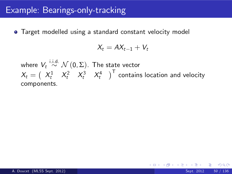
Example: Bearings-only-tracking
Target modelled using a standard constant velocity model Xt = AXt
i.i.d. 1
+ Vt
where Vt N (0, ). The state vector T 1 contains location and velocity Xt = Xt Xt2 Xt3 Xt4 components.
A. Doucet (MLSS Sept. 2012)
Sept. 2012
59 / 136
181
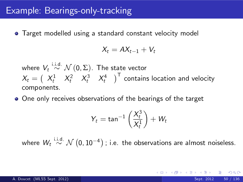
Example: Bearings-only-tracking
Target modelled using a standard constant velocity model Xt = AXt
i.i.d. 1
+ Vt
where Vt N (0, ). The state vector T 1 contains location and velocity Xt = Xt Xt2 Xt3 Xt4 components. One only receives observations of the bearings of the target Yt = tan where Wt
i.i.d. 1
Xt3 Xt1
+ Wt
N 0, 10
4
; i.e. the observations are almost noiseless.
A. Doucet (MLSS Sept. 2012)
Sept. 2012
59 / 136
182
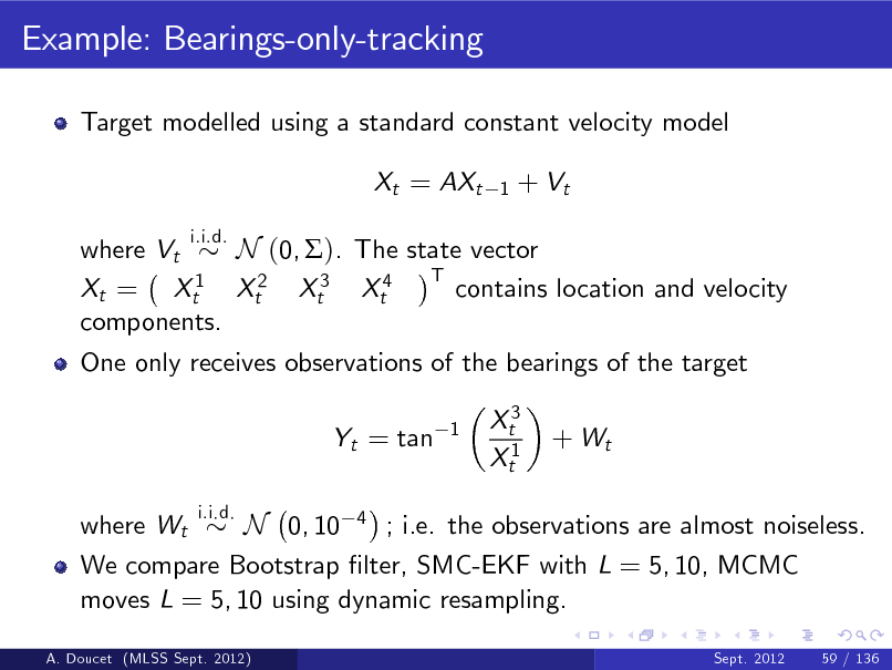
Example: Bearings-only-tracking
Target modelled using a standard constant velocity model Xt = AXt
i.i.d. 1
+ Vt
where Vt N (0, ). The state vector T 1 contains location and velocity Xt = Xt Xt2 Xt3 Xt4 components. One only receives observations of the bearings of the target Yt = tan where Wt
i.i.d. 1
Xt3 Xt1
+ Wt
N 0, 10 4 ; i.e. the observations are almost noiseless. We compare Bootstrap lter, SMC-EKF with L = 5, 10, MCMC moves L = 5, 10 using dynamic resampling.
Sept. 2012 59 / 136
A. Doucet (MLSS Sept. 2012)
183
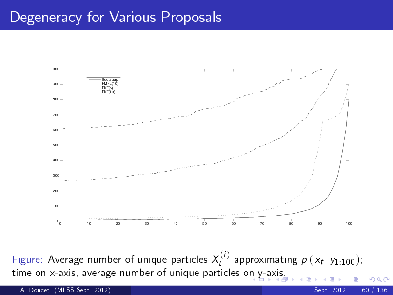
Degeneracy for Various Proposals
1000 Bootstrap RMFL(10) EKF(5) EKF(10)
900
800
700
600
500
400
300
200
100
0
0
10
20
30
40
50
60
70
80
90
100
Figure: Average number of unique particles Xt approximating p ( xt j y1 :100 ); time on x-axis, average number of unique particles on y-axis.
A. Doucet (MLSS Sept. 2012) Sept. 2012 60 / 136
(i )
184
Summary
SMC provide consistent estimates under weak assumptions.
A. Doucet (MLSS Sept. 2012)
Sept. 2012
61 / 136
185
Summary
SMC provide consistent estimates under weak assumptions. We can estimate fp ( xt j y1:t )gt 1 satisfactorily but our approximations of fp ( x1:t j y1:t )gt 1 degenerates as t increases because of resampling steps.
A. Doucet (MLSS Sept. 2012)
Sept. 2012
61 / 136
186
Summary
SMC provide consistent estimates under weak assumptions. We can estimate fp ( xt j y1:t )gt 1 satisfactorily but our approximations of fp ( x1:t j y1:t )gt 1 degenerates as t increases because of resampling steps. Resampling is crucial.
A. Doucet (MLSS Sept. 2012)
Sept. 2012
61 / 136
187
Summary
SMC provide consistent estimates under weak assumptions. We can estimate fp ( xt j y1:t )gt 1 satisfactorily but our approximations of fp ( x1:t j y1:t )gt 1 degenerates as t increases because of resampling steps. Resampling is crucial. We can mitigate but not eliminate the degeneracy problem by the design of clever proposals.
A. Doucet (MLSS Sept. 2012)
Sept. 2012
61 / 136
188
Summary
SMC provide consistent estimates under weak assumptions. We can estimate fp ( xt j y1:t )gt 1 satisfactorily but our approximations of fp ( x1:t j y1:t )gt 1 degenerates as t increases because of resampling steps. Resampling is crucial. We can mitigate but not eliminate the degeneracy problem by the design of clever proposals. Smoothing methods to estimate p ( x1:T j y1:T ) can come to the rescue.
A. Doucet (MLSS Sept. 2012)
Sept. 2012
61 / 136
189
Smoothing in State-Space Models
Smoothing problem: given a xed time T , we are interested in p ( x1:T j y1:T ) or some of its marginals, e.g. fp ( xt j y1:T )gT=1 . t
A. Doucet (MLSS Sept. 2012)
Sept. 2012
62 / 136
190
Smoothing in State-Space Models
Smoothing problem: given a xed time T , we are interested in p ( x1:T j y1:T ) or some of its marginals, e.g. fp ( xt j y1:T )gT=1 . t Smoothing is crucial to parameter estimation.
A. Doucet (MLSS Sept. 2012)
Sept. 2012
62 / 136
191
Smoothing in State-Space Models
Smoothing problem: given a xed time T , we are interested in p ( x1:T j y1:T ) or some of its marginals, e.g. fp ( xt j y1:T )gT=1 . t Smoothing is crucial to parameter estimation. Direct SMC approximations of p ( x1:T j y1:T ) and its marginals p ( xk j y1:T ) are poor if T is large.
A. Doucet (MLSS Sept. 2012)
Sept. 2012
62 / 136
192
Smoothing in State-Space Models
Smoothing problem: given a xed time T , we are interested in p ( x1:T j y1:T ) or some of its marginals, e.g. fp ( xt j y1:T )gT=1 . t Smoothing is crucial to parameter estimation. Direct SMC approximations of p ( x1:T j y1:T ) and its marginals p ( xk j y1:T ) are poor if T is large.
SMC provide good approximations of marginals fp ( xt j y1:t )gt This can be used to develop e cient smoothing estimates. Fixed-lag smoothing Forward-backward smoothing (Generalized) two-lter smoothing
1.
A. Doucet (MLSS Sept. 2012)
Sept. 2012
62 / 136
193
Fixed-Lag Smoothing
The xed-lag smoothing approximation relies on p ( xt j y1:T ) p ( xt j y1:t + ) for large enough.
and quantitative bounds can be established under stability assumptions.
A. Doucet (MLSS Sept. 2012)
Sept. 2012
63 / 136
194
Fixed-Lag Smoothing
The xed-lag smoothing approximation relies on p ( xt j y1:T ) p ( xt j y1:t + ) for large enough.
and quantitative bounds can be established under stability assumptions. This can be exploited by SMC methods (Kitagawa & Sato, 2001)
A. Doucet (MLSS Sept. 2012)
Sept. 2012
63 / 136
195
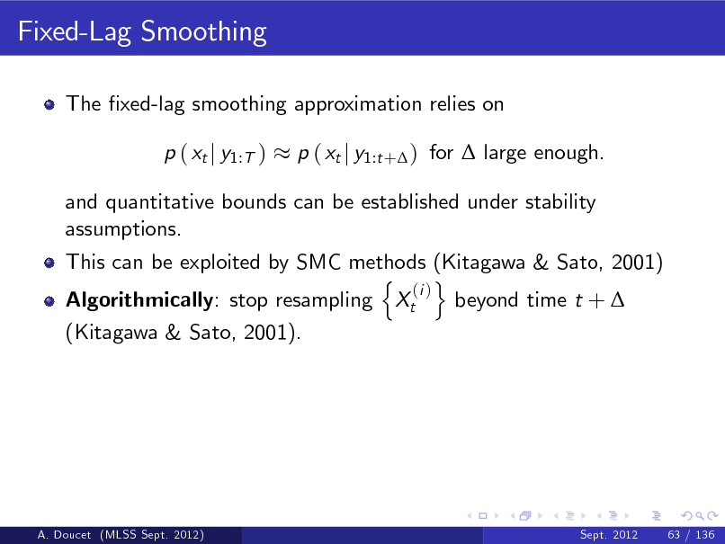
Fixed-Lag Smoothing
The xed-lag smoothing approximation relies on p ( xt j y1:T ) p ( xt j y1:t + ) for large enough.
and quantitative bounds can be established under stability assumptions. This can be exploited by SMC methods (Kitagawa & Sato, 2001) n o (i ) Algorithmically: stop resampling Xt beyond time t + (Kitagawa & Sato, 2001).
A. Doucet (MLSS Sept. 2012)
Sept. 2012
63 / 136
196
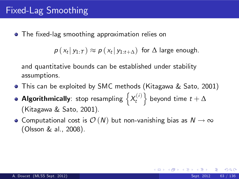
Fixed-Lag Smoothing
The xed-lag smoothing approximation relies on p ( xt j y1:T ) p ( xt j y1:t + ) for large enough.
and quantitative bounds can be established under stability assumptions. This can be exploited by SMC methods (Kitagawa & Sato, 2001) n o (i ) Algorithmically: stop resampling Xt beyond time t + (Kitagawa & Sato, 2001). Computational cost is O (N ) but non-vanishing bias as N ! (Olsson & al., 2008).
A. Doucet (MLSS Sept. 2012)
Sept. 2012
63 / 136
197
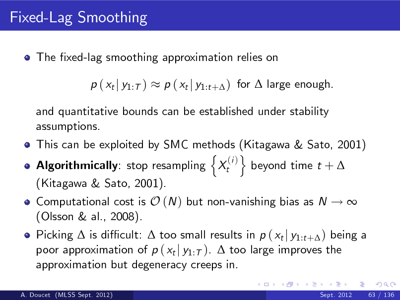
Fixed-Lag Smoothing
The xed-lag smoothing approximation relies on p ( xt j y1:T ) p ( xt j y1:t + ) for large enough.
and quantitative bounds can be established under stability assumptions. This can be exploited by SMC methods (Kitagawa & Sato, 2001) n o (i ) Algorithmically: stop resampling Xt beyond time t + (Kitagawa & Sato, 2001). Computational cost is O (N ) but non-vanishing bias as N ! (Olsson & al., 2008). Picking is di cult: too small results in p ( xt j y1:t + ) being a poor approximation of p ( xt j y1:T ). too large improves the approximation but degeneracy creeps in.
A. Doucet (MLSS Sept. 2012) Sept. 2012 63 / 136
198
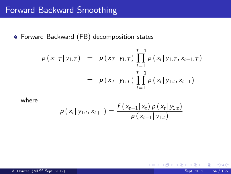
Forward Backward Smoothing
Forward Backward (FB) decomposition states
T
p ( x1:T j y1:T ) = p ( xT j y1:T )
t =1 T 1 t =1
p ( xt j y1:T , xt +1:T ) p ( xt j y1:t , xt +1 )
1
= p ( xT j y1:T )
where p ( xt j y1:t , xt +1 ) =
f ( xt +1 j xt ) p ( xt j y1:t ) . p ( xt +1 j y1:t )
A. Doucet (MLSS Sept. 2012)
Sept. 2012
64 / 136
199
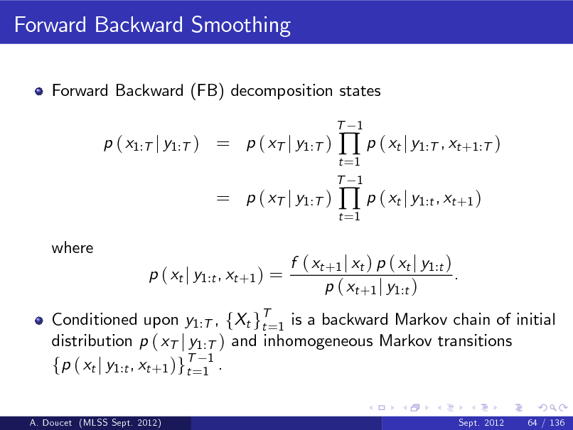
Forward Backward Smoothing
Forward Backward (FB) decomposition states
T
p ( x1:T j y1:T ) = p ( xT j y1:T )
t =1 T 1 t =1
p ( xt j y1:T , xt +1:T ) p ( xt j y1:t , xt +1 )
1
= p ( xT j y1:T )
where p ( xt j y1:t , xt +1 ) =
Conditioned upon y1:T , fXt gT=1 is a backward Markov chain of initial t distribution p ( xT j y1:T ) and inhomogeneous Markov transitions fp ( xt j y1:t , xt +1 )gT=11 . t
A. Doucet (MLSS Sept. 2012) Sept. 2012 64 / 136
f ( xt +1 j xt ) p ( xt j y1:t ) . p ( xt +1 j y1:t )
200
Forward Filtering Backward Sampling
To obtain a sample from p ( x1:T j y1:T ) ,
A. Doucet (MLSS Sept. 2012)
Sept. 2012
65 / 136
201
Forward Filtering Backward Sampling
To obtain a sample from p ( x1:T j y1:T ) ,
Forward ltering: compute and store fp ( xt j y1 :t )gT=1 t
A. Doucet (MLSS Sept. 2012)
Sept. 2012
65 / 136
202
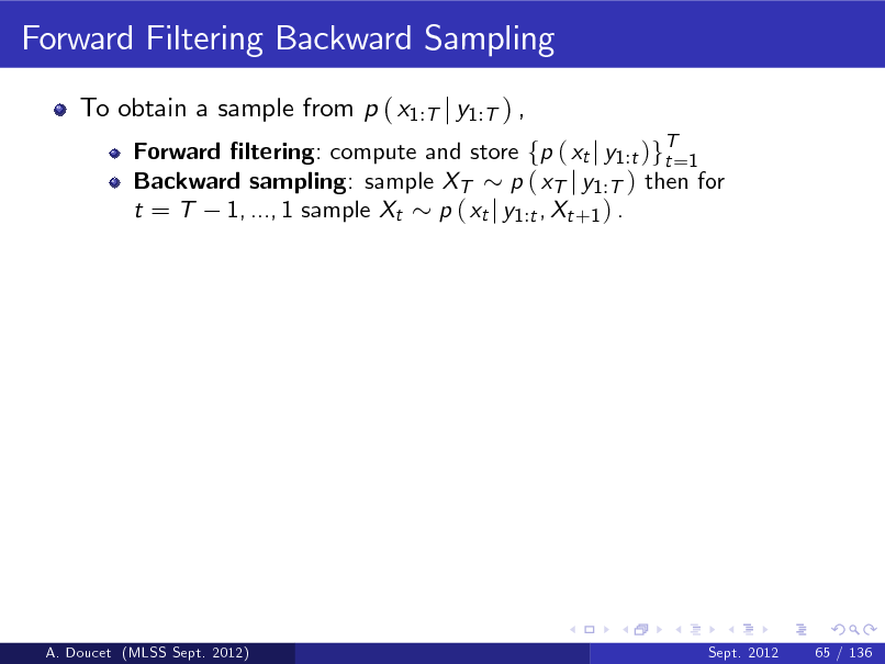
Forward Filtering Backward Sampling
To obtain a sample from p ( x1:T j y1:T ) ,
Forward ltering: compute and store fp ( xt j y1 :t )gT=1 t Backward sampling: sample XT p ( xT j y1 :T ) then for t = T 1, ..., 1 sample Xt p ( xt j y1 :t , Xt +1 ) .
A. Doucet (MLSS Sept. 2012)
Sept. 2012
65 / 136
203
Forward Filtering Backward Sampling
To obtain a sample from p ( x1:T j y1:T ) ,
Forward ltering: compute and store fp ( xt j y1 :t )gT=1 t Backward sampling: sample XT p ( xT j y1 :T ) then for t = T 1, ..., 1 sample Xt p ( xt j y1 :t , Xt +1 ) .
SMC to obtain an approximate sample from p ( x1:T j y1:T )
A. Doucet (MLSS Sept. 2012)
Sept. 2012
65 / 136
204
Forward Filtering Backward Sampling
To obtain a sample from p ( x1:T j y1:T ) ,
Forward ltering: compute and store fp ( xt j y1 :t )gT=1 t Backward sampling: sample XT p ( xT j y1 :T ) then for t = T 1, ..., 1 sample Xt p ( xt j y1 :t , Xt +1 ) . Forward ltering: compute and store fp ( xt j y1 :t )gT=1 . b t
SMC to obtain an approximate sample from p ( x1:T j y1:T )
A. Doucet (MLSS Sept. 2012)
Sept. 2012
65 / 136
205
Forward Filtering Backward Sampling
To obtain a sample from p ( x1:T j y1:T ) ,
Forward ltering: compute and store fp ( xt j y1 :t )gT=1 t Backward sampling: sample XT p ( xT j y1 :T ) then for t = T 1, ..., 1 sample Xt p ( xt j y1 :t , Xt +1 ) . Forward ltering: compute and store fp ( xt j y1 :t )gT=1 . b t Backward sampling: sample XT p ( xT j y1 :T ) then for b t = T 1, ..., 1 sample Xt p ( xt j y1 :t , Xt +1 ) where b p ( xt j y1 :t , Xt +1 ) b f ( Xt +1 j xt ) p ( xt j y1 :t ) b
i =1
SMC to obtain an approximate sample from p ( x1:T j y1:T )
f
N
Xt +1 j Xt
(i )
Xt
(i )
( xt )
A. Doucet (MLSS Sept. 2012)
Sept. 2012
65 / 136
206
Forward Filtering Backward Sampling
To obtain a sample from p ( x1:T j y1:T ) ,
Forward ltering: compute and store fp ( xt j y1 :t )gT=1 t Backward sampling: sample XT p ( xT j y1 :T ) then for t = T 1, ..., 1 sample Xt p ( xt j y1 :t , Xt +1 ) . Forward ltering: compute and store fp ( xt j y1 :t )gT=1 . b t Backward sampling: sample XT p ( xT j y1 :T ) then for b t = T 1, ..., 1 sample Xt p ( xt j y1 :t , Xt +1 ) where b p ( xt j y1 :t , Xt +1 ) b f ( Xt +1 j xt ) p ( xt j y1 :t ) b
i =1
SMC to obtain an approximate sample from p ( x1:T j y1:T )
f
N
Xt +1 j Xt
(i )
Xt
(i )
( xt )
Direct implementation O (NT ) (Godsill, D. & West, 2004). Rejection sampling possible if f ( xt +1 j xt ) C (xt +1 ) (Douc et al., 2011) and cost O (NT ) .
A. Doucet (MLSS Sept. 2012) Sept. 2012 65 / 136
207
Forward Filtering Backward Smoothing
Assume you want to compute the marginal smoothing distributions fp ( xt j y1:T )gT=1 instead of sampling from them. t
A. Doucet (MLSS Sept. 2012)
Sept. 2012
66 / 136
208
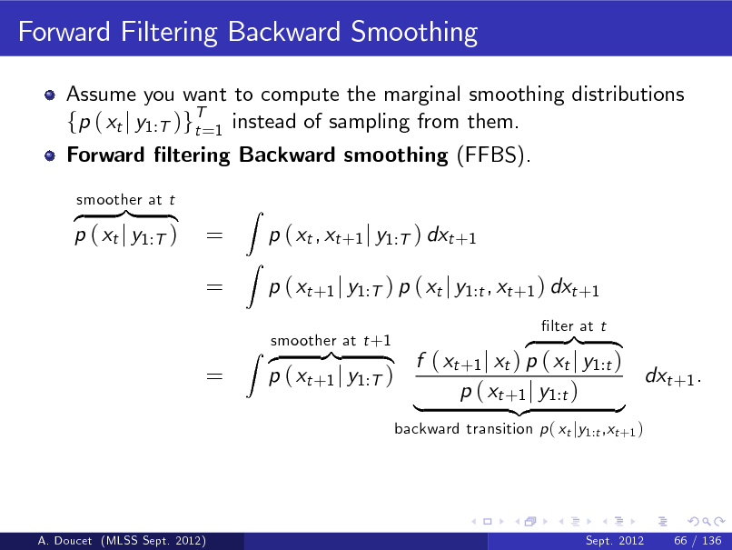
Forward Filtering Backward Smoothing
Assume you want to compute the marginal smoothing distributions fp ( xt j y1:T )gT=1 instead of sampling from them. t Forward ltering Backward smoothing (FFBS). z }| { p ( xt j y1:T )
smoother at t
= =
Z Z
p ( xt , xt +1 j y1:T ) dxt +1 p ( xt +1 j y1:T ) p ( xt j y1:t , xt +1 ) dxt +1 z }| { f ( xt +1 j xt ) p ( xt j y1:t ) dxt +1 . p ( xt +1 j y1:T ) p ( xt +1 j y1:t ) | {z }
backward transition p ( xt jy1:t ,xt +1 ) lter at t
=
smoother at t +1 Z z }| {
A. Doucet (MLSS Sept. 2012)
Sept. 2012
66 / 136
209
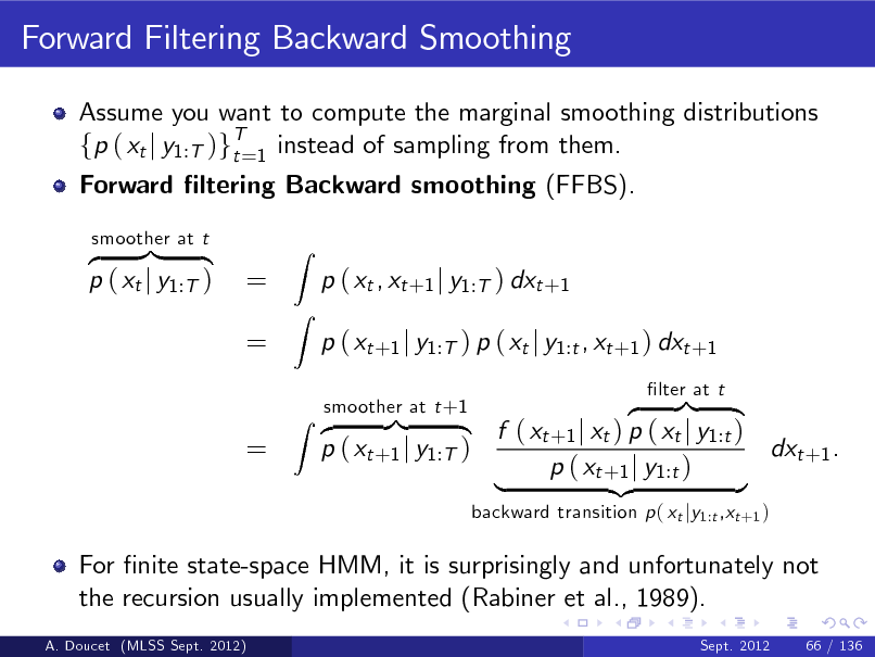
Forward Filtering Backward Smoothing
Assume you want to compute the marginal smoothing distributions fp ( xt j y1:T )gT=1 instead of sampling from them. t Forward ltering Backward smoothing (FFBS). z }| { p ( xt j y1:T )
smoother at t
= =
Z Z
p ( xt , xt +1 j y1:T ) dxt +1 p ( xt +1 j y1:T ) p ( xt j y1:t , xt +1 ) dxt +1 z }| { f ( xt +1 j xt ) p ( xt j y1:t ) dxt +1 . p ( xt +1 j y1:T ) p ( xt +1 j y1:t ) | {z }
backward transition p ( xt jy1:t ,xt +1 ) lter at t
=
smoother at t +1 Z z }| {
For nite state-space HMM, it is surprisingly and unfortunately not the recursion usually implemented (Rabiner et al., 1989).
A. Doucet (MLSS Sept. 2012) Sept. 2012
66 / 136
210
SMC Forward Filtering Backward Smoothing
Forward ltering: compute and store fp ( xt j y1:t )gT=1 using your b t favourite SMC.
A. Doucet (MLSS Sept. 2012)
Sept. 2012
67 / 136
211
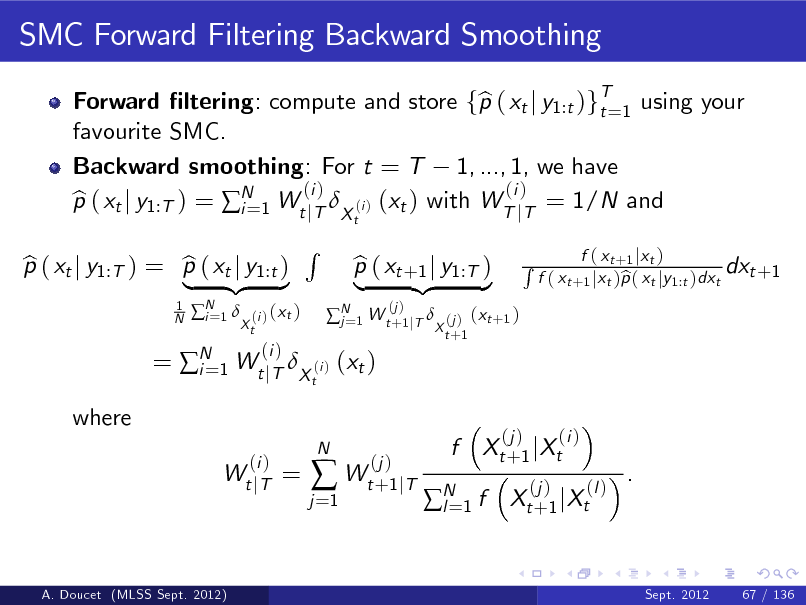
SMC Forward Filtering Backward Smoothing
Forward ltering: compute and store fp ( xt j y1:t )gT=1 using your b t favourite SMC. Backward smoothing: For t = T 1, ..., 1, we have (i ) (i ) p ( xt j y1:T ) = N 1 Wt jT X (i ) (xt ) with WT jT = 1/N and b i=
t 1 N
p ( xt j y1:T ) = p ( xt j y1:t ) b b | {z }
N 1 i=
(i ) ( x t ) Xt
R
t
N 1 W t +1 jT j=
= N 1 Wt jT X (i ) (xt ) i=
(i ) Wt j T
(i )
p ( xt +1 j y1:T ) b | {z }
(j )
(j ) ( x t +1 ) X t +1
R
f ( x t +1 j x t ) dxt +1 f ( xt +1 jxt )p ( xt jy1:t )dxt b
where
=
j =1
N
(j ) Wt +1 jT
f
Xt + 1 j Xt
(j )
(j )
(i ) (l )
N 1 f l=
.
Xt + 1 j Xt
A. Doucet (MLSS Sept. 2012)
Sept. 2012
67 / 136
212
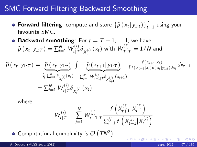
SMC Forward Filtering Backward Smoothing
Forward ltering: compute and store fp ( xt j y1:t )gT=1 using your b t favourite SMC. Backward smoothing: For t = T 1, ..., 1, we have (i ) (i ) p ( xt j y1:T ) = N 1 Wt jT X (i ) (xt ) with WT jT = 1/N and b i=
t 1 N
p ( xt j y1:T ) = p ( xt j y1:t ) b b | {z }
N 1 i=
(i ) ( x t ) Xt
R
t
N 1 W t +1 jT j=
= N 1 Wt jT X (i ) (xt ) i=
(i ) Wt j T
(i )
p ( xt +1 j y1:T ) b | {z }
(j )
(j ) ( x t +1 ) X t +1
R
f ( x t +1 j x t ) dxt +1 f ( xt +1 jxt )p ( xt jy1:t )dxt b
where
=
j =1
N
(j ) Wt +1 jT
f
Xt + 1 j Xt
(j )
(j )
(i ) (l )
N 1 f l=
.
Xt + 1 j Xt
Computational complexity is O TN 2 .
A. Doucet (MLSS Sept. 2012) Sept. 2012 67 / 136
213

Two-Filter Smoothing
An alternative to FB smoothing is the Two-Filter (TF) formula z }| { z }| { p ( xt , xt +1 j y1:T ) p ( xt j y1:t )f ( xt +1 j xt ) p ( yt +1:T j xt +1 )
forward lter backward lter
A. Doucet (MLSS Sept. 2012)
Sept. 2012
68 / 136
214
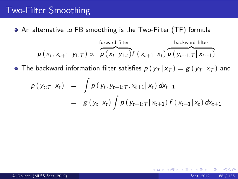
Two-Filter Smoothing
An alternative to FB smoothing is the Two-Filter (TF) formula z }| { z }| { p ( xt , xt +1 j y1:T ) p ( xt j y1:t )f ( xt +1 j xt ) p ( yt +1:T j xt +1 )
Z
forward lter backward lter
The backward information lter satises p ( yT j xT ) = g ( yT j xT ) and p ( yt :T j xt ) = p ( yt , yt +1:T , xt +1 j xt ) dxt +1
Z
= g ( yt j xt )
p ( yt +1:T j xt +1 ) f ( xt +1 j xt ) dxt +1
A. Doucet (MLSS Sept. 2012)
Sept. 2012
68 / 136
215
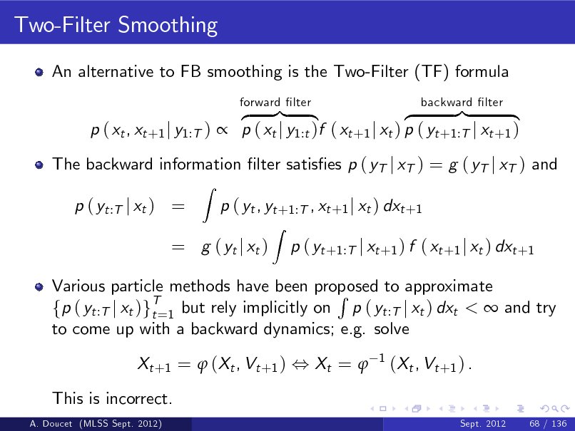
Two-Filter Smoothing
An alternative to FB smoothing is the Two-Filter (TF) formula z }| { z }| { p ( xt , xt +1 j y1:T ) p ( xt j y1:t )f ( xt +1 j xt ) p ( yt +1:T j xt +1 )
Z
forward lter backward lter
The backward information lter satises p ( yT j xT ) = g ( yT j xT ) and p ( yt :T j xt ) = p ( yt , yt +1:T , xt +1 j xt ) dxt +1
Z
= g ( yt j xt )
p ( yt +1:T j xt +1 ) f ( xt +1 j xt ) dxt +1
Various particle methods have been proposed to approximate R fp ( yt :T j xt )gT=1 but rely implicitly on p ( yt :T j xt ) dxt < and try t to come up with a backward dynamics; e.g. solve Xt + 1 = ( Xt , Vt + 1 ) , Xt = This is incorrect.
A. Doucet (MLSS Sept. 2012) Sept. 2012 68 / 136
1
( Xt , Vt + 1 ) .
216
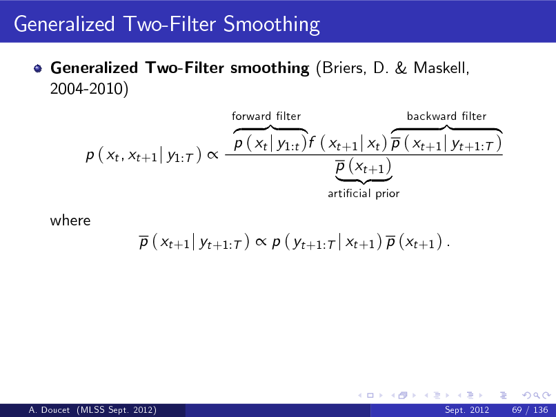
Generalized Two-Filter Smoothing
Generalized Two-Filter smoothing (Briers, D. & Maskell, 2004-2010) z }| { }| { z p ( xt j y1:t )f ( xt +1 j xt ) p ( xt +1 j yt +1:T ) p ( xt , xt +1 j y1:T ) p (xt +1 ) | {z }
articial prior forward lter backward lter
where
p ( xt +1 j yt +1:T ) p ( yt +1:T j xt +1 ) p (xt +1 ) .
A. Doucet (MLSS Sept. 2012)
Sept. 2012
69 / 136
217
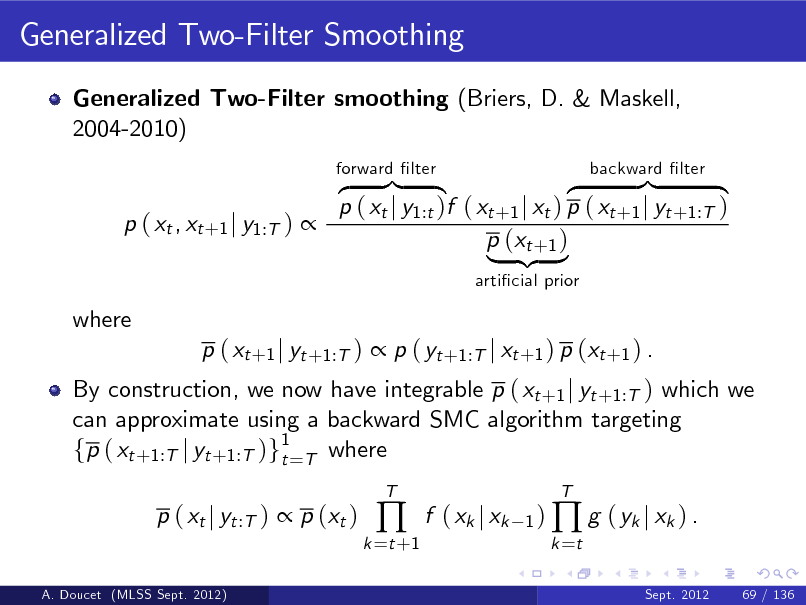
Generalized Two-Filter Smoothing
Generalized Two-Filter smoothing (Briers, D. & Maskell, 2004-2010) z }| { }| { z p ( xt j y1:t )f ( xt +1 j xt ) p ( xt +1 j yt +1:T ) p ( xt , xt +1 j y1:T ) p (xt +1 ) | {z }
articial prior forward lter backward lter
where
By construction, we now have integrable p ( xt +1 j yt +1:T ) which we can approximate using a backward SMC algorithm targeting fp ( xt +1:T j yt +1:T )g1=T where t p ( xt j yt :T ) p (xt )
A. Doucet (MLSS Sept. 2012)
p ( xt +1 j yt +1:T ) p ( yt +1:T j xt +1 ) p (xt +1 ) .
k =t +1
T
f ( xk j xk
1 ) g ( yk j xk ) . k =t
Sept. 2012 69 / 136
T
218
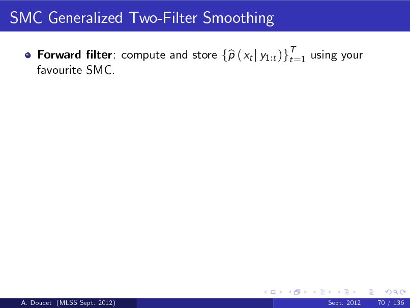
SMC Generalized Two-Filter Smoothing
Forward lter: compute and store fp ( xt j y1:t )gT=1 using your b t favourite SMC.
A. Doucet (MLSS Sept. 2012)
Sept. 2012
70 / 136
219
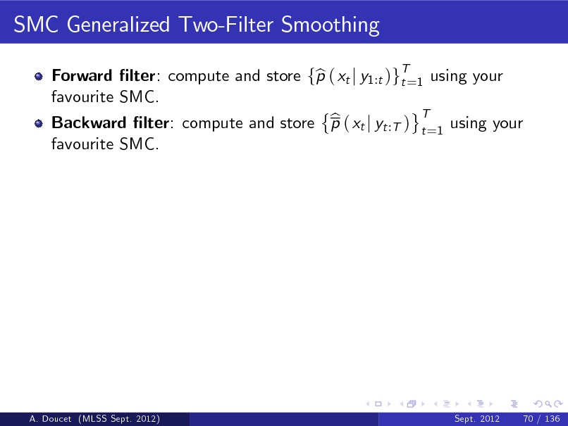
SMC Generalized Two-Filter Smoothing
Forward lter: compute and store fp ( xt j y1:t )gT=1 using your b t favourite SMC. T b Backward lter: compute and store p ( xt j yt :T ) t =1 using your favourite SMC.
A. Doucet (MLSS Sept. 2012)
Sept. 2012
70 / 136
220
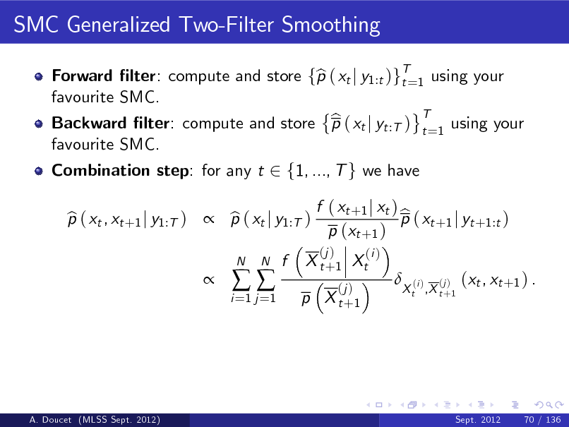
SMC Generalized Two-Filter Smoothing
Forward lter: compute and store fp ( xt j y1:t )gT=1 using your b t favourite SMC. T b Backward lter: compute and store p ( xt j yt :T ) t =1 using your favourite SMC. Combination step: for any t 2 f1, ..., T g we have p ( xt , xt +1 j y1:T ) p ( xt j y1:T ) b b
i =1 j =1
N
N
f
X t + 1 Xt
(j )
f ( xt +1 j xt ) b p ( xt +1 j yt +1:t ) p (xt +1 )
(j ) (i )
p X t +1
X t ,X t +1
(i )
(j )
(xt , xt +1 ) .
A. Doucet (MLSS Sept. 2012)
Sept. 2012
70 / 136
221
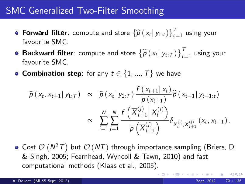
SMC Generalized Two-Filter Smoothing
Forward lter: compute and store fp ( xt j y1:t )gT=1 using your b t favourite SMC. T b Backward lter: compute and store p ( xt j yt :T ) t =1 using your favourite SMC. Combination step: for any t 2 f1, ..., T g we have p ( xt , xt +1 j y1:T ) p ( xt j y1:T ) b b
i =1 j =1
N
N
f
X t + 1 Xt
(j )
f ( xt +1 j xt ) b p ( xt +1 j yt +1:t ) p (xt +1 )
(j ) (i )
p X t +1
X t ,X t +1
(i )
(j )
(xt , xt +1 ) .
Cost O N 2 T but O (NT ) through importance sampling (Briers, D. & Singh, 2005; Fearnhead, Wyncoll & Tawn, 2010) and fast computational methods (Klaas et al., 2005).
A. Doucet (MLSS Sept. 2012) Sept. 2012 70 / 136
222
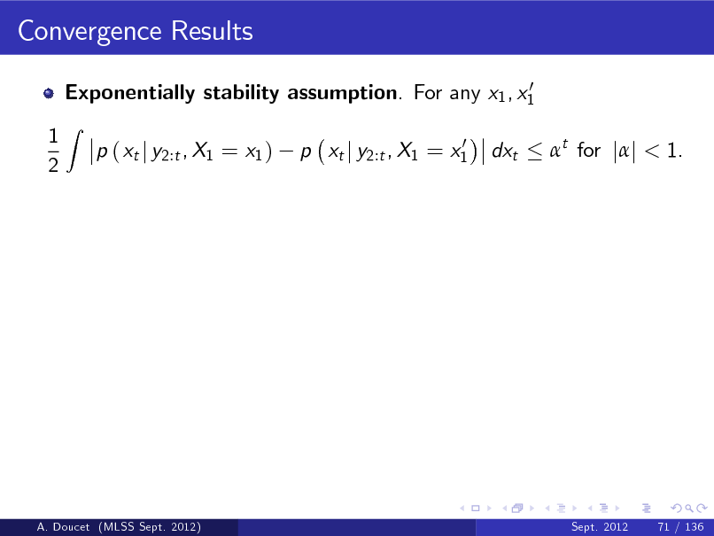
Convergence Results
0 Exponentially stability assumption. For any x1 , x1
1 2
Z
p ( xt j y2:t , X1 = x1 )
0 p xt j y2:t , X1 = x1
dxt
t for jj < 1.
A. Doucet (MLSS Sept. 2012)
Sept. 2012
71 / 136
223
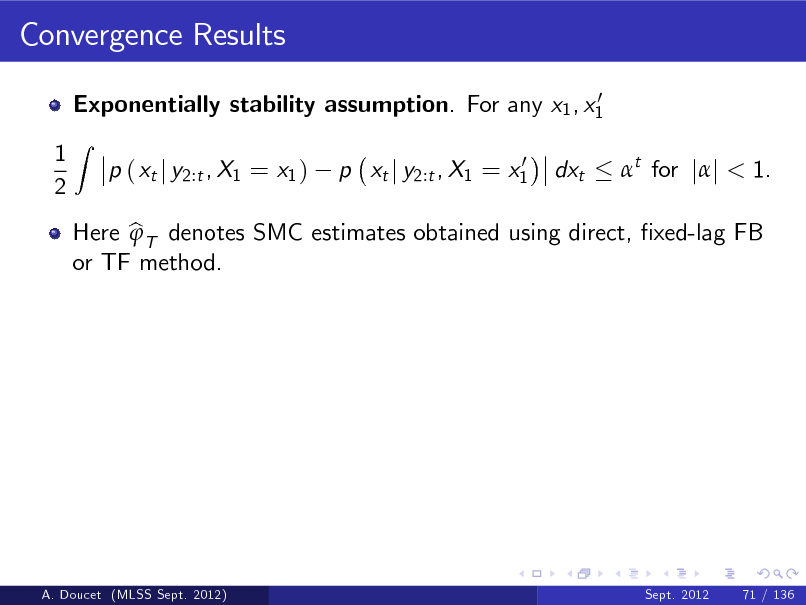
Convergence Results
0 Exponentially stability assumption. For any x1 , x1
1 2
Z
p ( xt j y2:t , X1 = x1 )
0 p xt j y2:t , X1 = x1
dxt
t for jj < 1.
Here b T denotes SMC estimates obtained using direct, xed-lag FB or TF method.
A. Doucet (MLSS Sept. 2012)
Sept. 2012
71 / 136
224
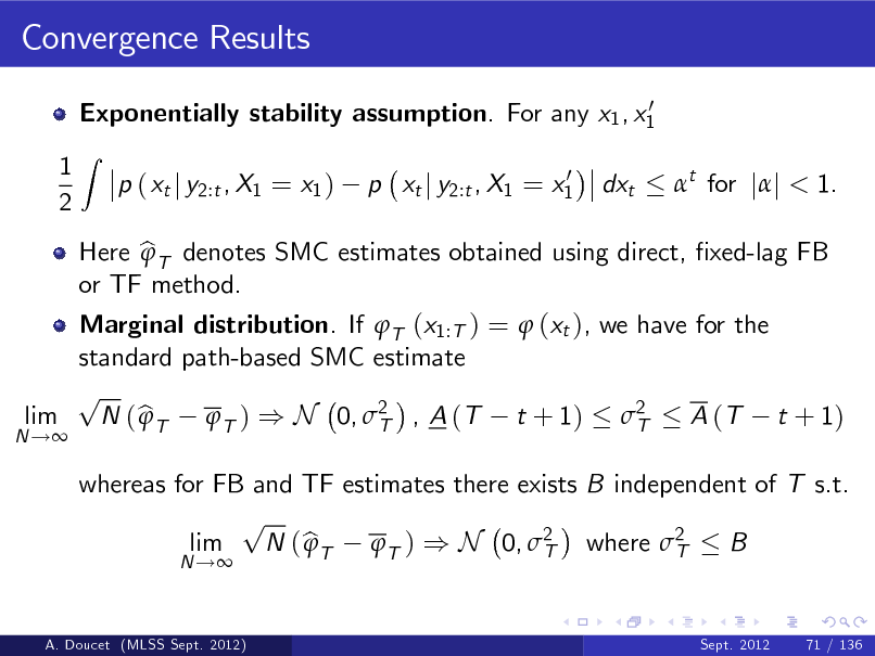
Convergence Results
0 Exponentially stability assumption. For any x1 , x1
1 2
Z
p ( xt j y2:t , X1 = x1 )
0 p xt j y2:t , X1 = x1
dxt
t for jj < 1.
N !
Marginal distribution. If T (x1:T ) = (xt ), we have for the standard path-based SMC estimate p lim N ( b T T ) ) N 0, 2 , A (T t + 1) 2 A (T t + 1) T T
N !
Here b T denotes SMC estimates obtained using direct, xed-lag FB or TF method.
whereas for FB and TF estimates there exists B independent of T s.t. p lim N ( b T T ) ) N 0, 2 where 2 B T T
Sept. 2012 71 / 136
A. Doucet (MLSS Sept. 2012)
225
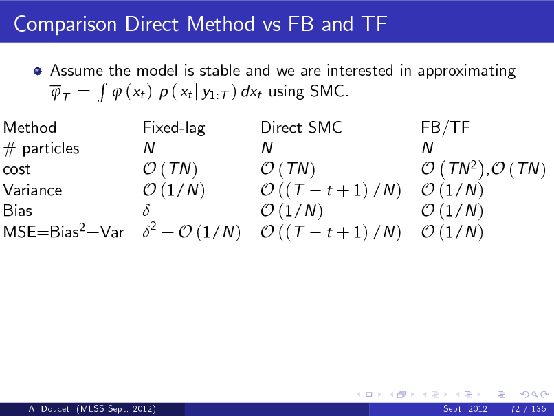
Comparison Direct Method vs FB and TF
Assume the model is stable and we are interested in approximating R T = (xt ) p ( xt j y1:T ) dxt using SMC. Fixed-lag N O (TN ) O (1/N ) 2 + O (1/N ) Direct SMC N O (TN ) O ((T t + 1) /N ) O (1/N ) O ((T t + 1) /N )
Method # particles cost Variance Bias MSE=Bias2 +Var
FB/TF N O TN 2 ,O (TN ) O (1/N ) O (1/N ) O (1/N )
A. Doucet (MLSS Sept. 2012)
Sept. 2012
72 / 136
226
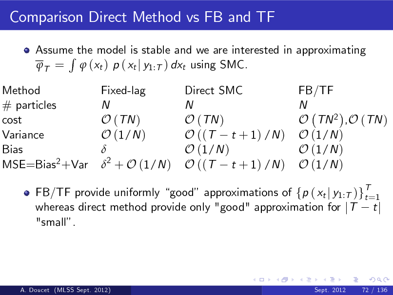
Comparison Direct Method vs FB and TF
Assume the model is stable and we are interested in approximating R T = (xt ) p ( xt j y1:T ) dxt using SMC. Fixed-lag N O (TN ) O (1/N ) 2 + O (1/N ) Direct SMC N O (TN ) O ((T t + 1) /N ) O (1/N ) O ((T t + 1) /N )
Method # particles cost Variance Bias MSE=Bias2 +Var
FB/TF N O TN 2 ,O (TN ) O (1/N ) O (1/N ) O (1/N )
FB/TF provide uniformly good approximations of fp ( xt j y1:T )gT=1 t whereas direct method provide only "good" approximation for jT t j "small.
A. Doucet (MLSS Sept. 2012)
Sept. 2012
72 / 136
227
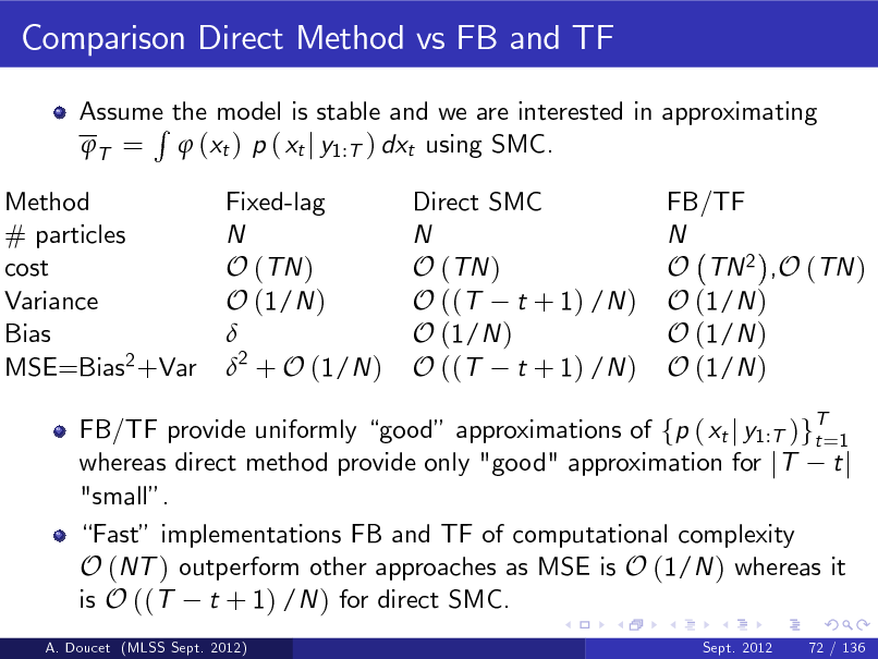
Comparison Direct Method vs FB and TF
Assume the model is stable and we are interested in approximating R T = (xt ) p ( xt j y1:T ) dxt using SMC. Fixed-lag N O (TN ) O (1/N ) 2 + O (1/N ) Direct SMC N O (TN ) O ((T t + 1) /N ) O (1/N ) O ((T t + 1) /N )
Method # particles cost Variance Bias MSE=Bias2 +Var
FB/TF N O TN 2 ,O (TN ) O (1/N ) O (1/N ) O (1/N )
FB/TF provide uniformly good approximations of fp ( xt j y1:T )gT=1 t whereas direct method provide only "good" approximation for jT t j "small. Fast implementations FB and TF of computational complexity O (NT ) outperform other approaches as MSE is O (1/N ) whereas it is O ((T t + 1) /N ) for direct SMC.
A. Doucet (MLSS Sept. 2012) Sept. 2012 72 / 136
228
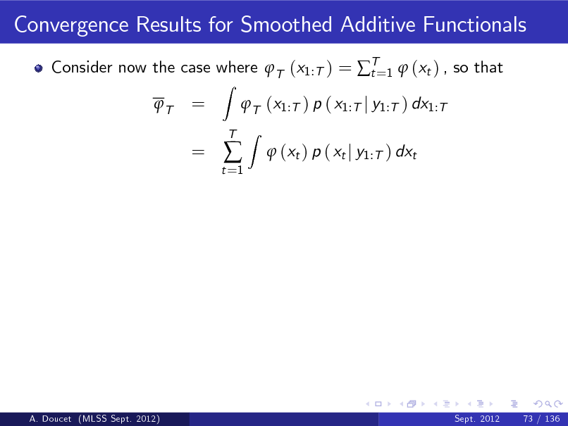
Convergence Results for Smoothed Additive Functionals
Consider now the case where T (x1:T ) = T=1 (xt ) , so that t T
Z
= =
T (x1:T ) p ( x1:T j y1:T ) dx1:T
Z
t =1
T
(xt ) p ( xt j y1:T ) dxt
A. Doucet (MLSS Sept. 2012)
Sept. 2012
73 / 136
229
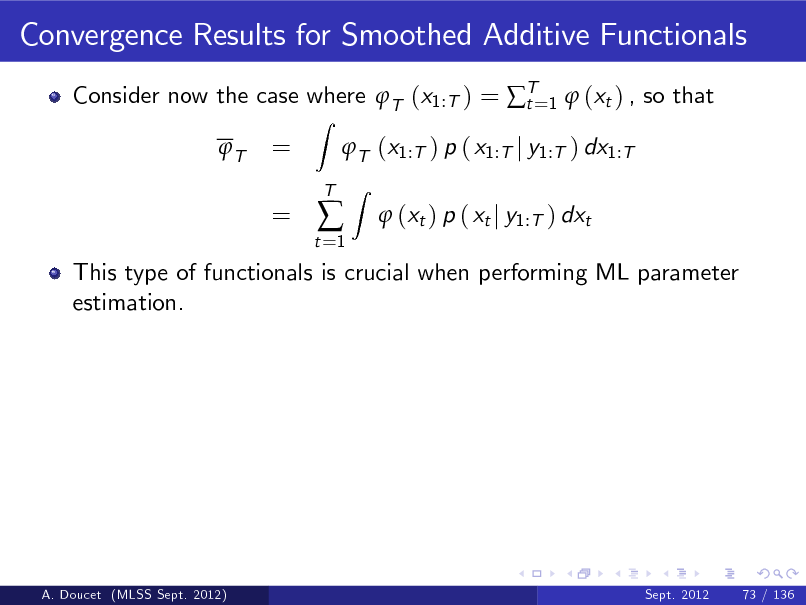
Convergence Results for Smoothed Additive Functionals
Consider now the case where T (x1:T ) = T=1 (xt ) , so that t T
Z
= =
T (x1:T ) p ( x1:T j y1:T ) dx1:T
Z
t =1
T
(xt ) p ( xt j y1:T ) dxt
This type of functionals is crucial when performing ML parameter estimation.
A. Doucet (MLSS Sept. 2012)
Sept. 2012
73 / 136
230
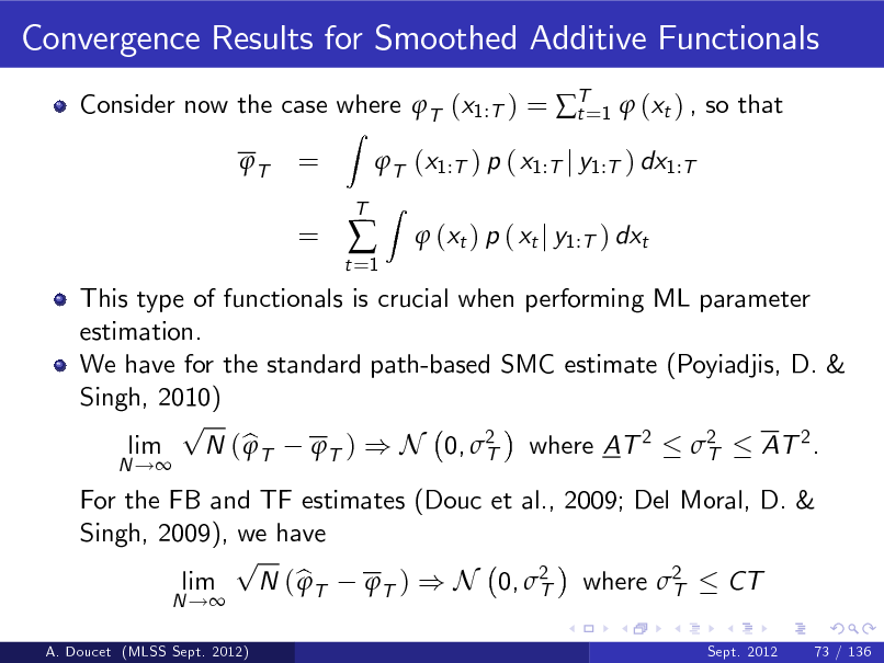
Convergence Results for Smoothed Additive Functionals
Consider now the case where T (x1:T ) = T=1 (xt ) , so that t T
Z
= =
T (x1:T ) p ( x1:T j y1:T ) dx1:T
Z
t =1
T
(xt ) p ( xt j y1:T ) dxt
A. Doucet (MLSS Sept. 2012)
For the FB and TF estimates (Douc et al., 2009; Del Moral, D. & Singh, 2009), we have p lim N ( b T T ) ) N 0, 2 where 2 CT T T
N !
Sept. 2012
This type of functionals is crucial when performing ML parameter estimation. We have for the standard path-based SMC estimate (Poyiadjis, D. & Singh, 2010) p lim N ( b T T ) ) N 0, 2 where AT 2 2 AT 2 . T T
N !
73 / 136
231
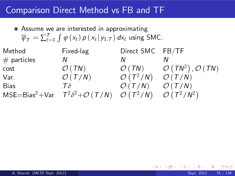
Comparison Direct Method vs FB and TF
Assume we are interested in approximating R T = T=1 (xt ) p ( xt j y1:T ) dxt using SMC. t Fixed-lag N O (TN ) O (T /N ) T T 2 2 +O (T /N ) Direct SMC N O (TN ) O T 2 /N O (T /N ) O T 2 /N
Method # particles cost Var. Bias MSE=Bias2 +Var
FB/TF N O TN 2 , O (TN ) O (T /N ) O (T /N ) O T 2 /N 2
A. Doucet (MLSS Sept. 2012)
Sept. 2012
74 / 136
232
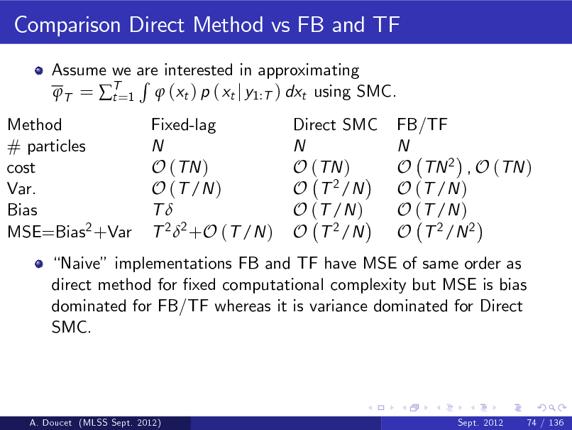
Comparison Direct Method vs FB and TF
Assume we are interested in approximating R T = T=1 (xt ) p ( xt j y1:T ) dxt using SMC. t Fixed-lag N O (TN ) O (T /N ) T T 2 2 +O (T /N ) Direct SMC N O (TN ) O T 2 /N O (T /N ) O T 2 /N
Method # particles cost Var. Bias MSE=Bias2 +Var
FB/TF N O TN 2 , O (TN ) O (T /N ) O (T /N ) O T 2 /N 2
Naive implementations FB and TF have MSE of same order as direct method for xed computational complexity but MSE is bias dominated for FB/TF whereas it is variance dominated for Direct SMC.
A. Doucet (MLSS Sept. 2012)
Sept. 2012
74 / 136
233
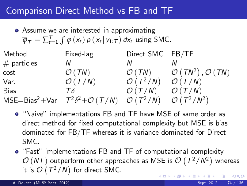
Comparison Direct Method vs FB and TF
Assume we are interested in approximating R T = T=1 (xt ) p ( xt j y1:T ) dxt using SMC. t Fixed-lag N O (TN ) O (T /N ) T T 2 2 +O (T /N ) Direct SMC N O (TN ) O T 2 /N O (T /N ) O T 2 /N
Method # particles cost Var. Bias MSE=Bias2 +Var
FB/TF N O TN 2 , O (TN ) O (T /N ) O (T /N ) O T 2 /N 2
Naive implementations FB and TF have MSE of same order as direct method for xed computational complexity but MSE is bias dominated for FB/TF whereas it is variance dominated for Direct SMC. Fast implementations FB and TF of computational complexity O (NT ) outperform other approaches as MSE is O T 2 /N 2 whereas it is O T 2 /N for direct SMC.
A. Doucet (MLSS Sept. 2012) Sept. 2012 74 / 136
234
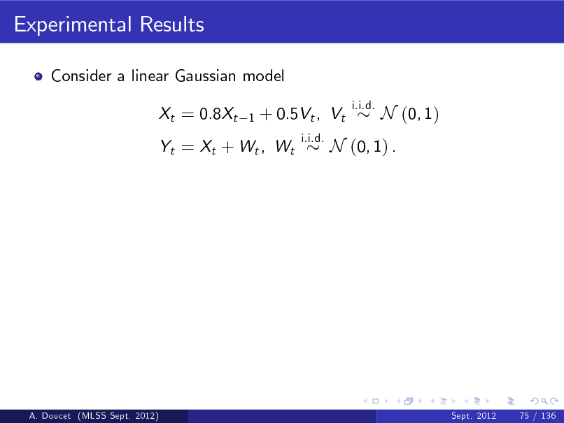
Experimental Results
Consider a linear Gaussian model Xt = 0.8Xt
1
+ 0.5Vt , Vt
i.i.d.
i.i.d.
N (0, 1)
Yt = Xt + Wt , Wt
N (0, 1) .
A. Doucet (MLSS Sept. 2012)
Sept. 2012
75 / 136
235
![Slide: Experimental Results
Consider a linear Gaussian model Xt = 0.8Xt
1
+ 0.5Vt , Vt
i.i.d.
i.i.d.
N (0, 1)
Yt = Xt + Wt , Wt
N (0, 1) .
We simulate 10,000 observations and compute SMC estimates of
Z
T (x1:T ) p ( x1:T j y1:T ) dx1:T
for 4 dierent additive functionals t (x1:t ) = t 1 (x1:t 1 ) + (xt 1 , xt , yt ) including 1 (xt 1 , xt , yt ) = xt 1 xt , 2 (xt 1 , xt , yt ) = xt2 . [Ground truth can be computed using Kalman smoother.]
A. Doucet (MLSS Sept. 2012)
Sept. 2012
75 / 136](https://yosinski.com/mlss12/media/slides/MLSS-2012-Doucet-Sequential-Monte-Carlo-Methods_236.png)
Experimental Results
Consider a linear Gaussian model Xt = 0.8Xt
1
+ 0.5Vt , Vt
i.i.d.
i.i.d.
N (0, 1)
Yt = Xt + Wt , Wt
N (0, 1) .
We simulate 10,000 observations and compute SMC estimates of
Z
T (x1:T ) p ( x1:T j y1:T ) dx1:T
for 4 dierent additive functionals t (x1:t ) = t 1 (x1:t 1 ) + (xt 1 , xt , yt ) including 1 (xt 1 , xt , yt ) = xt 1 xt , 2 (xt 1 , xt , yt ) = xt2 . [Ground truth can be computed using Kalman smoother.]
A. Doucet (MLSS Sept. 2012)
Sept. 2012
75 / 136
236
![Slide: Experimental Results
Consider a linear Gaussian model Xt = 0.8Xt
1
+ 0.5Vt , Vt
i.i.d.
i.i.d.
N (0, 1)
Yt = Xt + Wt , Wt
N (0, 1) .
We simulate 10,000 observations and compute SMC estimates of
Z
T (x1:T ) p ( x1:T j y1:T ) dx1:T
for 4 dierent additive functionals t (x1:t ) = t 1 (x1:t 1 ) + (xt 1 , xt , yt ) including 1 (xt 1 , xt , yt ) = xt 1 xt , 2 (xt 1 , xt , yt ) = xt2 . [Ground truth can be computed using Kalman smoother.] We use SMC over 100 replications on the same dataset to estimate the empirical variance.
A. Doucet (MLSS Sept. 2012) Sept. 2012 75 / 136](https://yosinski.com/mlss12/media/slides/MLSS-2012-Doucet-Sequential-Monte-Carlo-Methods_237.png)
Experimental Results
Consider a linear Gaussian model Xt = 0.8Xt
1
+ 0.5Vt , Vt
i.i.d.
i.i.d.
N (0, 1)
Yt = Xt + Wt , Wt
N (0, 1) .
We simulate 10,000 observations and compute SMC estimates of
Z
T (x1:T ) p ( x1:T j y1:T ) dx1:T
for 4 dierent additive functionals t (x1:t ) = t 1 (x1:t 1 ) + (xt 1 , xt , yt ) including 1 (xt 1 , xt , yt ) = xt 1 xt , 2 (xt 1 , xt , yt ) = xt2 . [Ground truth can be computed using Kalman smoother.] We use SMC over 100 replications on the same dataset to estimate the empirical variance.
A. Doucet (MLSS Sept. 2012) Sept. 2012 75 / 136
237
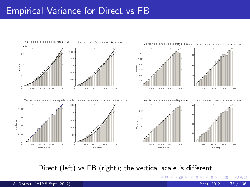
Empirical Variance for Direct vs FB
V a r ia n c e o f s c o r e e s tim a te w .r .t.
x 10 10000 6 8000
4
v
V a r ia n c e o f s c o r e e s tim a te w .r .t.
V a r ia n c e o f s c o r e e s tim a te w .r .t.
v
V a r ia n c e o f s c o r e e s tim a te w .r .t.
120 100
60
V a ri a n c e
6000
V ariance
4
80 60 40
40
4000 2 2000
20
20 0 0 0 0
0 0
2500
5000
7500
10000
0 0
2500
5000
7500
10000
2500
5000
7500
10000
2500
5000
7500
10000
V a r ia n c e o f s c o r e e s tim a te w .r .t.
w
V a r ia n c e o f s c o r e e s tim a te w .r .t. c
V a r ia n c e o f s c o r e e s tim a te w .r .t.
w
V a r ia n c e o f s c o r e e s tim a te w .r .t. c
5000 4000 20 4000
40
30 3000
V a ri a n c e
V ariance
3000 2000 2000
15 20 10
1000
1000
5
10
0 0
2500
5000
7500
10000
0 0
2500
5000
7500
10000
0 0
2500
5000
7500
10000
0 0
2500
5000
7500
10000
T i m e s te p s
T i m e s te p s
T i m e s te p s
T i m e s te p s
Direct (left) vs FB (right); the vertical scale is dierent
A. Doucet (MLSS Sept. 2012) Sept. 2012 76 / 136
238
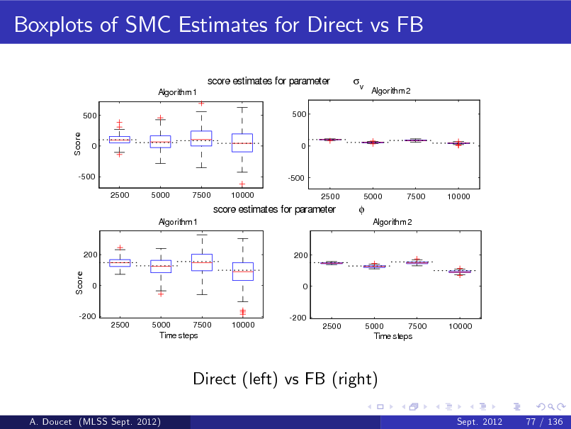
Boxplots of SMC Estimates for Direct vs FB
score estimates for parameter
Algorithm 1
500 500
v
Algorithm 2
Score
0
0
-500 2500 5000 7500 10000
-500 2500 5000 7500 10000
score estimates for parameter
Algorithm 1
Algorithm 2
200
200
Score
0
0
-200 2500 5000 7500 10000
-200 2500 5000 7500 10000
Time steps
Time steps
Direct (left) vs FB (right)
A. Doucet (MLSS Sept. 2012) Sept. 2012 77 / 136
239

Summary
SMC smoothing techniques allow us to solve the degeneracy problem.
A. Doucet (MLSS Sept. 2012)
Sept. 2012
78 / 136
240
Summary
SMC smoothing techniques allow us to solve the degeneracy problem. SMC xed-lag smoothing is the simplest one but has non-vanishing bias di cult to quantify.
A. Doucet (MLSS Sept. 2012)
Sept. 2012
78 / 136
241
Summary
SMC smoothing techniques allow us to solve the degeneracy problem. SMC xed-lag smoothing is the simplest one but has non-vanishing bias di cult to quantify. SMC FB and SMC TF algorithms provide uniformly good approximations of marginal smoothing distributions contrary to direct method.
A. Doucet (MLSS Sept. 2012)
Sept. 2012
78 / 136
242
Summary
SMC smoothing techniques allow us to solve the degeneracy problem. SMC xed-lag smoothing is the simplest one but has non-vanishing bias di cult to quantify. SMC FB and SMC TF algorithms provide uniformly good approximations of marginal smoothing distributions contrary to direct method. In terms of MSE, only fast implementations of SMC FB/TF provide a gain in terms of MSE.
A. Doucet (MLSS Sept. 2012)
Sept. 2012
78 / 136
243
Summary
SMC smoothing techniques allow us to solve the degeneracy problem. SMC xed-lag smoothing is the simplest one but has non-vanishing bias di cult to quantify. SMC FB and SMC TF algorithms provide uniformly good approximations of marginal smoothing distributions contrary to direct method. In terms of MSE, only fast implementations of SMC FB/TF provide a gain in terms of MSE. For direct implementation SMC FB/TF, MSE is of the same order but SMC FB/TF is bias dominated and direct SMC is variance dominated.
A. Doucet (MLSS Sept. 2012)
Sept. 2012
78 / 136
244
ML Parameter Estimation in State-Space Models
In most scenarios of interest, the state-space model contains an unknown static parameter 2 so that X1 (x1 ) and Xt j (Xt
1
= xt
1)
f ( xt j xt
1) .
A. Doucet (MLSS Sept. 2012)
Sept. 2012
79 / 136
245
ML Parameter Estimation in State-Space Models
In most scenarios of interest, the state-space model contains an unknown static parameter 2 so that X1 (x1 ) and Xt j (Xt
1
= xt
1)
f ( xt j xt
1) .
The observations fYt gt 1 are conditionally independent given fXt gt 1 and Yt j (Xt = xt ) g ( yt j xt ) .
A. Doucet (MLSS Sept. 2012)
Sept. 2012
79 / 136
246
ML Parameter Estimation in State-Space Models
In most scenarios of interest, the state-space model contains an unknown static parameter 2 so that X1 (x1 ) and Xt j (Xt
1
= xt
1)
f ( xt j xt
1) .
The observations fYt gt 1 are conditionally independent given fXt gt 1 and Yt j (Xt = xt ) g ( yt j xt ) . In many applications, we actually only care about and would like to estimate it o-line or on-line.
A. Doucet (MLSS Sept. 2012)
Sept. 2012
79 / 136
247
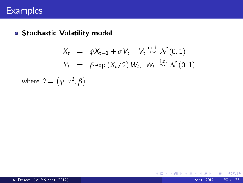
Examples
Stochastic Volatility model Xt Yt
= Xt
1
+ Vt , Vt
i.i.d.
= exp (Xt /2) Wt , Wt
i.i.d.
N (0, 1) N (0, 1)
where = , 2 , .
A. Doucet (MLSS Sept. 2012)
Sept. 2012
80 / 136
248
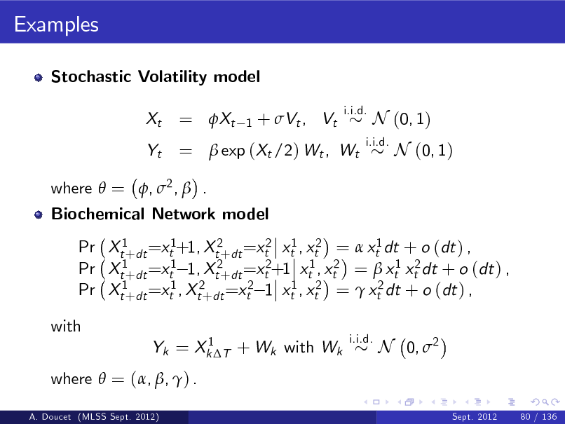
Examples
Stochastic Volatility model Xt Yt
= Xt
1
+ Vt , Vt
i.i.d.
= exp (Xt /2) Wt , Wt
i.i.d.
N (0, 1) N (0, 1)
where = , 2 , . Biochemical Network model Pr Xt1+dt =xt1+1, Xt2+dt =xt2 xt1 , xt2 = xt1 dt + o (dt ) , Pr Xt1+dt =xt1 1, Xt2+dt =xt2+1 xt1 , xt2 = xt1 xt2 dt + o (dt ) , Pr Xt1+dt =xt1 , Xt2+dt =xt2 1 xt1 , xt2 = xt2 dt + o (dt ) , with
1 Yk = Xk T + Wk with Wk i.i.d.
N 0, 2
Sept. 2012 80 / 136
where = (, , ) .
A. Doucet (MLSS Sept. 2012)
249
Likelihood Function Estimation
Let y1:T being given, the log-(marginal) likelihood is given by
`( ) = log p (y1:T ) .
A. Doucet (MLSS Sept. 2012)
Sept. 2012
81 / 136
250
Likelihood Function Estimation
Let y1:T being given, the log-(marginal) likelihood is given by
`( ) = log p (y1:T ) .
For any 2 , one can estimate `( ) using standard SMC. methods, variance O (T /N ) .
A. Doucet (MLSS Sept. 2012)
Sept. 2012
81 / 136
251
Likelihood Function Estimation
Let y1:T being given, the log-(marginal) likelihood is given by
`( ) = log p (y1:T ) .
For any 2 , one can estimate `( ) using standard SMC. methods, variance O (T /N ) . Direct maximization of `( ) di cult as SMC estimate b ) is not a `( smooth function of even for xed random seed.
A. Doucet (MLSS Sept. 2012)
Sept. 2012
81 / 136
252
Likelihood Function Estimation
Let y1:T being given, the log-(marginal) likelihood is given by
`( ) = log p (y1:T ) .
For any 2 , one can estimate `( ) using standard SMC. methods, variance O (T /N ) . Direct maximization of `( ) di cult as SMC estimate b ) is not a `( smooth function of even for xed random seed. For dim (Xt ) = 1, we can obtain smooth estimate of log-likelihood function by using a smoothed resampling step (e.g. Pitt, 2002-2011); i.e. piecewise linear approximation of Pr ( Xt < x j y1:t ) .
A. Doucet (MLSS Sept. 2012)
Sept. 2012
81 / 136
253
Likelihood Function Estimation
Let y1:T being given, the log-(marginal) likelihood is given by
`( ) = log p (y1:T ) .
For any 2 , one can estimate `( ) using standard SMC. methods, variance O (T /N ) . Direct maximization of `( ) di cult as SMC estimate b ) is not a `( smooth function of even for xed random seed. For dim (Xt ) = 1, we can obtain smooth estimate of log-likelihood function by using a smoothed resampling step (e.g. Pitt, 2002-2011); i.e. piecewise linear approximation of Pr ( Xt < x j y1:t ) . For dim (Xt ) > 1, we can obtain estimates of `( ) highly positively correlated for neigbouring values in (e.g. Lee, 2008).
A. Doucet (MLSS Sept. 2012)
Sept. 2012
81 / 136
254
Gradient Ascent
To maximise `( ) w.r.t , use at iteration k + 1 k +1 = k + k r`( )j = k where r`( )j = k is the so-called score vector.
A. Doucet (MLSS Sept. 2012)
Sept. 2012
82 / 136
255
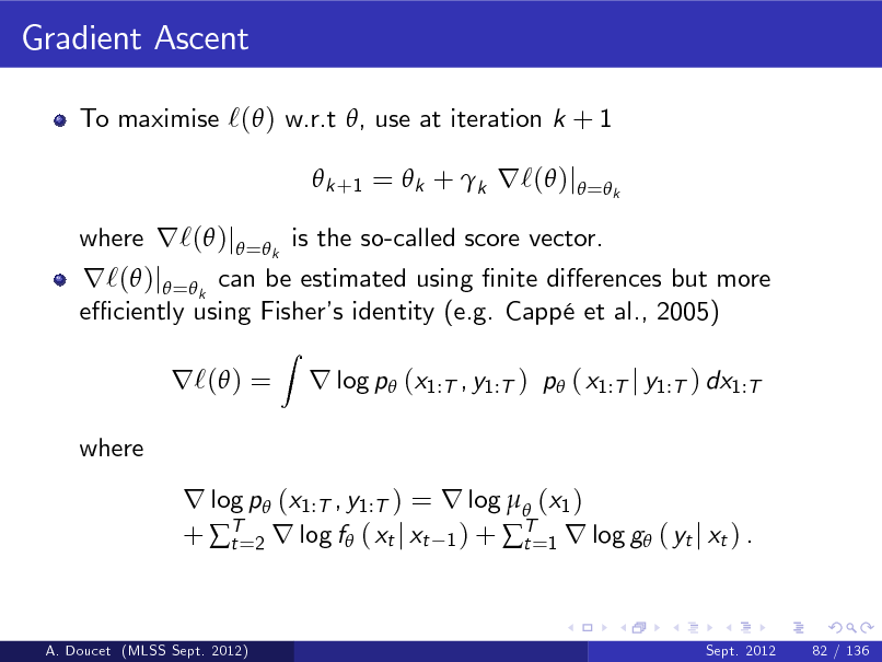
Gradient Ascent
To maximise `( ) w.r.t , use at iteration k + 1 k +1 = k + k r`( )j = k
r`( )j =k can be estimated using nite dierences but more e ciently using Fisher identity (e.g. Capp et al., 2005) s r`( ) =
where
Z
where r`( )j = k is the so-called score vector.
r log p (x1:T , y1:T ) p ( x1:T j y1:T ) dx1:T
r log p (x1:T , y1:T ) = r log (x1 ) + T=2 r log f ( xt j xt 1 ) + T=1 r log g ( yt j xt ) . t t
A. Doucet (MLSS Sept. 2012)
Sept. 2012
82 / 136
256
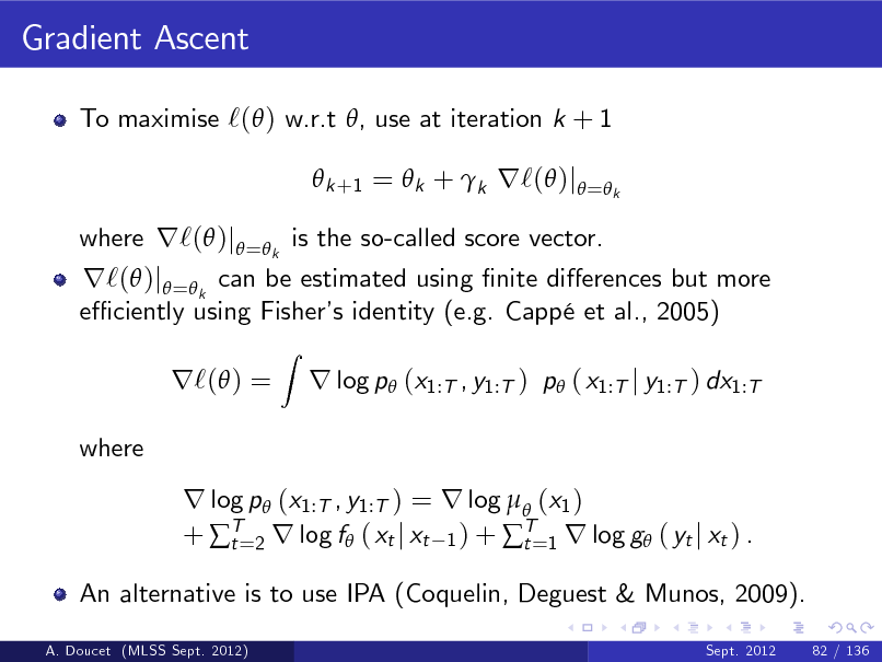
Gradient Ascent
To maximise `( ) w.r.t , use at iteration k + 1 k +1 = k + k r`( )j = k
r`( )j =k can be estimated using nite dierences but more e ciently using Fisher identity (e.g. Capp et al., 2005) s r`( ) =
where
Z
where r`( )j = k is the so-called score vector.
r log p (x1:T , y1:T ) p ( x1:T j y1:T ) dx1:T
r log p (x1:T , y1:T ) = r log (x1 ) + T=2 r log f ( xt j xt 1 ) + T=1 r log g ( yt j xt ) . t t
An alternative is to use IPA (Coquelin, Deguest & Munos, 2009).
A. Doucet (MLSS Sept. 2012) Sept. 2012 82 / 136
257
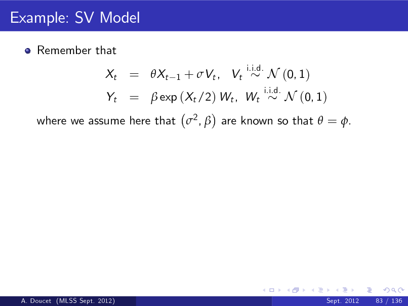
Example: SV Model
Remember that Xt Yt
i.i.d.
= Xt
1
+ Vt , Vt
= exp (Xt /2) Wt , Wt
i.i.d.
N (0, 1) N (0, 1)
where we assume here that 2 , are known so that = .
A. Doucet (MLSS Sept. 2012)
Sept. 2012
83 / 136
258
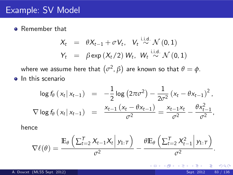
Example: SV Model
Remember that Xt Yt
i.i.d.
= Xt
1
+ Vt , Vt
= exp (Xt /2) Wt , Wt
i.i.d.
N (0, 1) N (0, 1)
where we assume here that 2 , are known so that = . In this scenario 1 1 log f ( xt j xt 1 ) = log 22 (xt xt 1 )2 , 2 2 2 xt2 1 xt 1 (xt xt 1 ) xt 1 xt r log f ( xt j xt 1 ) = = , 2 2 2 hence E T=2 Xt t 2
1 Xt
r`( ) =
y1:T
E T=2 Xt2 t 2
1
y1:T .
A. Doucet (MLSS Sept. 2012)
Sept. 2012
83 / 136
259
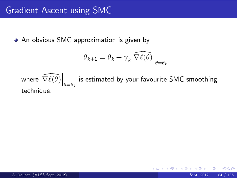
Gradient Ascent using SMC
An obvious SMC approximation is given by
\ k +1 = k + k r`( ) \ where r`( )
= k
= k
is estimated by your favourite SMC smoothing
technique.
A. Doucet (MLSS Sept. 2012)
Sept. 2012
84 / 136
260
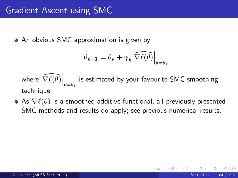
Gradient Ascent using SMC
An obvious SMC approximation is given by
\ k +1 = k + k r`( ) \ where r`( )
= k
= k
is estimated by your favourite SMC smoothing
technique.
As r`( ) is a smoothed additive functional, all previously presented SMC methods and results do apply; see previous numerical results.
A. Doucet (MLSS Sept. 2012)
Sept. 2012
84 / 136
261
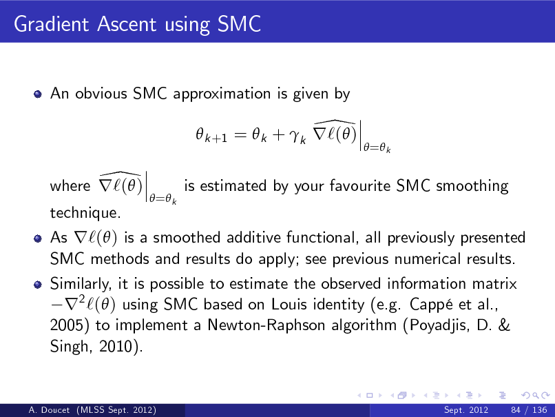
Gradient Ascent using SMC
An obvious SMC approximation is given by
\ k +1 = k + k r`( ) \ where r`( )
= k
= k
is estimated by your favourite SMC smoothing
technique.
As r`( ) is a smoothed additive functional, all previously presented SMC methods and results do apply; see previous numerical results. Similarly, it is possible to estimate the observed information matrix r2 `( ) using SMC based on Louis identity (e.g. Capp et al., 2005) to implement a Newton-Raphson algorithm (Poyadjis, D. & Singh, 2010).
A. Doucet (MLSS Sept. 2012)
Sept. 2012
84 / 136
262
ML Parameter Estimation using EM
The Expectation-Maximization (EM) algorithm is a celebrated alternative to gradient ascent technique.
A. Doucet (MLSS Sept. 2012)
Sept. 2012
85 / 136
263
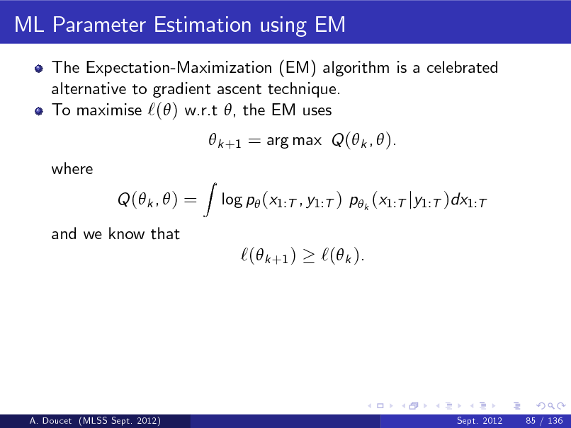
ML Parameter Estimation using EM
The Expectation-Maximization (EM) algorithm is a celebrated alternative to gradient ascent technique. To maximise `( ) w.r.t , the EM uses k +1 = arg max Q ( k , ). where Q ( k , ) = and we know that
Z
log p (x1:T , y1:T ) p k (x1:T jy1:T )dx1:T
`( k +1 )
`( k ).
A. Doucet (MLSS Sept. 2012)
Sept. 2012
85 / 136
264
ML Parameter Estimation using EM
The Expectation-Maximization (EM) algorithm is a celebrated alternative to gradient ascent technique. To maximise `( ) w.r.t , the EM uses k +1 = arg max Q ( k , ). where Q ( k , ) = and we know that
Z
log p (x1:T , y1:T ) p k (x1:T jy1:T )dx1:T
`( k +1 ) `( k ). If p (x1:T , y1:T ) is in the exponential family then we have
k +1 = T where
T =
A. Doucet (MLSS Sept. 2012)
1
Tk
Z
t =2
(xt
T
1 , xt , yt )
!
p (x1:T jy1:T )dx1:T
Sept. 2012 85 / 136
265
Example: SV Model
Remember that Xt Yt
i.i.d.
= Xt
1
+ Vt , Vt
= exp (Xt /2) Wt , Wt
i.i.d.
N (0, 1) N (0, 1)
where we assume here that 2 , are known so that = .
A. Doucet (MLSS Sept. 2012)
Sept. 2012
86 / 136
266
Example: SV Model
Remember that Xt Yt
i.i.d.
= Xt
1
+ Vt , Vt
= exp (Xt /2) Wt , Wt
i.i.d.
N (0, 1) N (0, 1)
where we assume here that 2 , are known so that = . In this scenario log f ( xt j xt
1)
= =
1 log 22 2 1 log 22 2 E k E k T=2 Xt t
1 (xt xt 1 )2 22 2 xt2 1 xt2 xt 1 xt + 2 2 2 2 2
1 Xt 1
so that k +1 = y1:T . y1:T
Sept. 2012 86 / 136
T=2 Xt2 t
A. Doucet (MLSS Sept. 2012)
267

EM using SMC
SMC approximation of the EM is direct.
A. Doucet (MLSS Sept. 2012)
Sept. 2012
87 / 136
268

EM using SMC
SMC approximation of the EM is direct. As EM requires computing smoothed additive functionals R T = T=2 (xt 1 , xt , yt ) p (x1:T jy1:T )dx1:T , all previously t presented SMC smoothing methods and results do apply.
A. Doucet (MLSS Sept. 2012)
Sept. 2012
87 / 136
269
EM using SMC
SMC approximation of the EM is direct. As EM requires computing smoothed additive functionals R T = T=2 (xt 1 , xt , yt ) p (x1:T jy1:T )dx1:T , all previously t presented SMC smoothing methods and results do apply.
There is obviously no more guarantee that `( k +1 ) `( k ) for nite N but many positive experimental results; e.g. (Schon, Wills & Ninness, 2011).
A. Doucet (MLSS Sept. 2012)
Sept. 2012
87 / 136
270

ML Parameter Estimation using Online Gradient
In many applications, we would like to estimate the parameter on-line.
A. Doucet (MLSS Sept. 2012)
Sept. 2012
88 / 136
271
ML Parameter Estimation using Online Gradient
In many applications, we would like to estimate the parameter on-line. Recursive maximum likelihood (Titterington, 1984; LeGland & Mevel, 1997) proceeds as follows t +1 = t + t r log p 1:t ( yt j y1:t
1)
where p 1:t ( yt j y1:t 1 ) is computed using k at time k and t t = , t 2 < . Under regularity conditions, this converges t towards a local maximum of the (average) log-likelihood.
A. Doucet (MLSS Sept. 2012)
Sept. 2012
88 / 136
272
ML Parameter Estimation using Online Gradient
In many applications, we would like to estimate the parameter on-line. Recursive maximum likelihood (Titterington, 1984; LeGland & Mevel, 1997) proceeds as follows t +1 = t + t r log p 1:t ( yt j y1:t
1)
where p 1:t ( yt j y1:t 1 ) is computed using k at time k and t t = , t 2 < . Under regularity conditions, this converges t towards a local maximum of the (average) log-likelihood. Note that
r log p1:t ( yt j y1:t
1)
= r log p1:t (y1:t )
r log p1:t
1
(y1:t
1)
is given by the dierence of two pseudo-score vectors where R r log p1:t (y1:t ) := t =2 r log f ( xk j xk 1 )j k k
A. Doucet (MLSS Sept. 2012)
+ r log g ( yk j xk )jk p1:t ( x1:t j y1:t ) dx1:t .
Sept. 2012 88 / 136
273
ML Parameter Estimation using SMC Online Gradient
SMC approximation follows
\ t +1 = t + t r log p 1:t ( yt j y1:t
where
1)
\ r log p 1:t ( yt j y1:t
1)
\ = r log p 1:t (y1:t )
\ r log p 1:t
1
(y1:t
1)
is given by the dierence of SMC estimates of pseudo-score vectors (Poyadjis, D. & Singh, 2011).
A. Doucet (MLSS Sept. 2012)
Sept. 2012
89 / 136
274
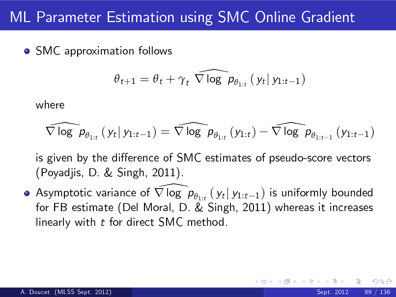
ML Parameter Estimation using SMC Online Gradient
SMC approximation follows
\ t +1 = t + t r log p 1:t ( yt j y1:t
where
1)
\ r log p 1:t ( yt j y1:t
1)
\ = r log p 1:t (y1:t )
\ r log p 1:t
1
(y1:t
1)
is given by the dierence of SMC estimates of pseudo-score vectors (Poyadjis, D. & Singh, 2011). \ Asymptotic variance of r log p 1:t ( yt j y1:t 1 ) is uniformly bounded for FB estimate (Del Moral, D. & Singh, 2011) whereas it increases linearly with t for direct SMC method.
A. Doucet (MLSS Sept. 2012)
Sept. 2012
89 / 136
275
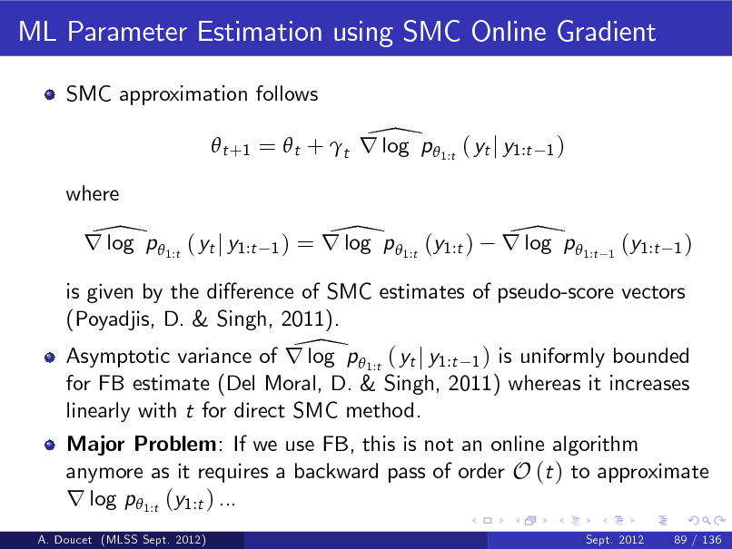
ML Parameter Estimation using SMC Online Gradient
SMC approximation follows
\ t +1 = t + t r log p 1:t ( yt j y1:t
where
1)
\ r log p 1:t ( yt j y1:t
1)
\ = r log p 1:t (y1:t )
\ r log p 1:t
1
(y1:t
1)
is given by the dierence of SMC estimates of pseudo-score vectors (Poyadjis, D. & Singh, 2011). \ Asymptotic variance of r log p 1:t ( yt j y1:t 1 ) is uniformly bounded for FB estimate (Del Moral, D. & Singh, 2011) whereas it increases linearly with t for direct SMC method. Major Problem: If we use FB, this is not an online algorithm anymore as it requires a backward pass of order O (t ) to approximate r log p1:t (y1:t ) ...
A. Doucet (MLSS Sept. 2012) Sept. 2012 89 / 136
276
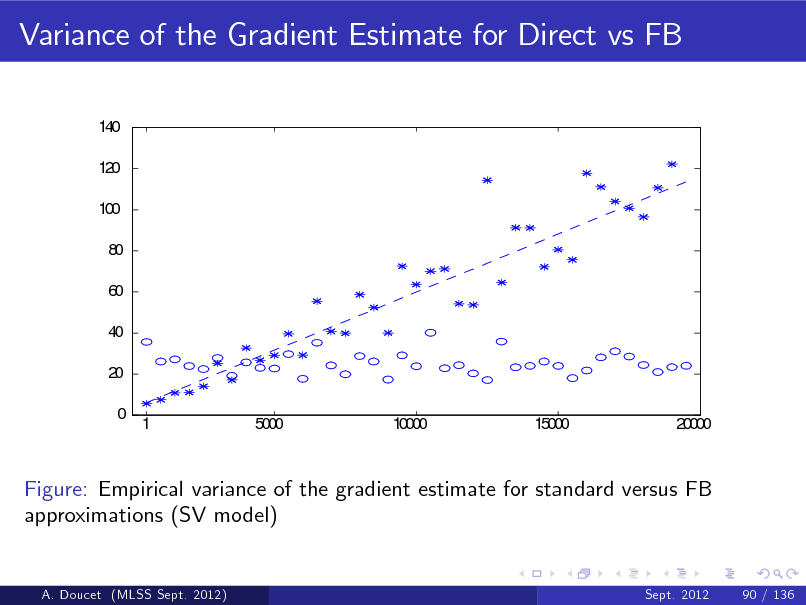
Variance of the Gradient Estimate for Direct vs FB
140 120 100 80 60 40 20 0 1 5000 10000 15000 20000
Figure: Empirical variance of the gradient estimate for standard versus FB approximations (SV model)
A. Doucet (MLSS Sept. 2012)
Sept. 2012
90 / 136
277
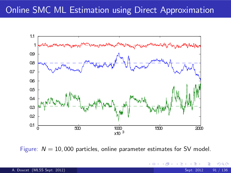
Online SMC ML Estimation using Direct Approximation
1.1 1 0.9 0.8 0.7 0.6 0.5 0.4 0.3 0.2 0.1 0 500 1000 x10 3 1500 2000
Figure: N = 10, 000 particles, online parameter estimates for SV model.
A. Doucet (MLSS Sept. 2012)
Sept. 2012
91 / 136
278
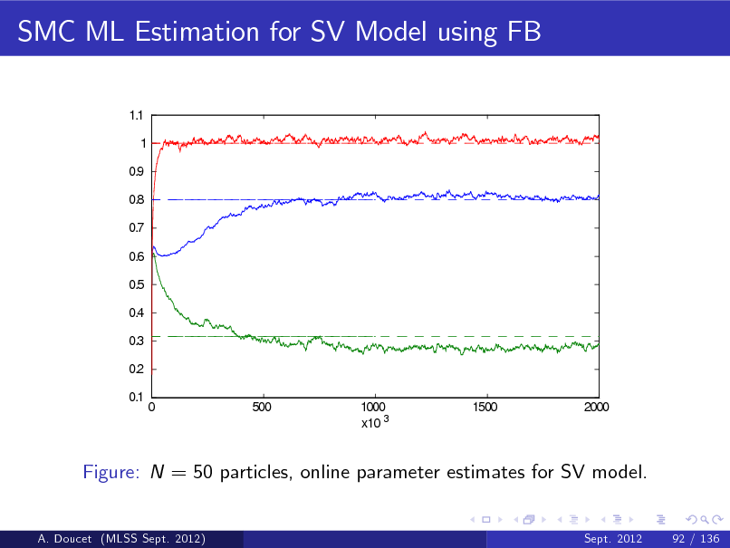
SMC ML Estimation for SV Model using FB
1.1 1 0.9 0.8 0.7 0.6 0.5 0.4 0.3 0.2 0.1 0 500 1000 x10 3 1500 2000
Figure: N = 50 particles, online parameter estimates for SV model.
A. Doucet (MLSS Sept. 2012)
Sept. 2012
92 / 136
279

Forward only Smoothing
For the time being, we do not have an online implementation as a backward pass of length t is required at time t.
A. Doucet (MLSS Sept. 2012)
Sept. 2012
93 / 136
280
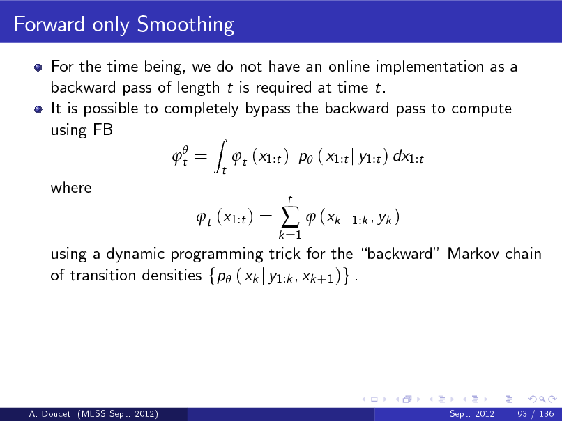
Forward only Smoothing
For the time being, we do not have an online implementation as a backward pass of length t is required at time t. It is possible to completely bypass the backward pass to compute using FB Z
t = t
t (x1:t ) p ( x1:t j y1:t ) dx1:t
where
t (x1:t ) =
k =1
(xk
t
1:k , yk )
using a dynamic programming trick for the backward Markov chain of transition densities fp ( xk j y1:k , xk +1 )g .
A. Doucet (MLSS Sept. 2012)
Sept. 2012
93 / 136
281
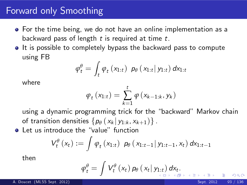
Forward only Smoothing
For the time being, we do not have an online implementation as a backward pass of length t is required at time t. It is possible to completely bypass the backward pass to compute using FB Z
t = t
t (x1:t ) p ( x1:t j y1:t ) dx1:t
where
t (x1:t ) =
k =1
(xk
t
1:k , yk )
using a dynamic programming trick for the backward Markov chain of transition densities fp ( xk j y1:k , xk +1 )g . Let us introduce the value function Vt (xt ) := then
A. Doucet (MLSS Sept. 2012)
Z
t (x1:t ) p ( x1:t
Z
1 j y1:t 1 , xt ) dx1:t 1
t =
Vt (xt ) p ( xt j y1:t ) dxt .
Sept. 2012 93 / 136
282
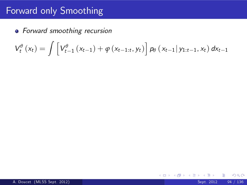
Forward only Smoothing
Forward smoothing recursion Z h Vt 1 (xt 1 ) + (xt Vt (xt ) = i , yt ) p ( xt 1:t
1 j y1:t 1 , xt ) dxt 1
A. Doucet (MLSS Sept. 2012)
Sept. 2012
94 / 136
283
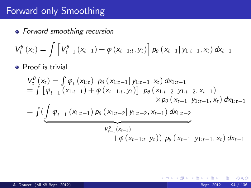
Forward only Smoothing
Forward smoothing recursion Z h Vt 1 (xt 1 ) + (xt Vt (xt ) = i , yt ) p ( xt 1:t
1 j y1:t 1 , xt ) dxt 1
Proof is trivial R VtR(xt ) = t (x1:t ) p ( x1:t 1 j y1:t 1 , xt ) dx1:t 1 = t 1 (x1:t 1 ) + (xt 1:t , yt ) p ( x1:t 2 j y1:t 2 , xt 1 ) p ( xt 1 j y1:t 1 , xt ) dx1:t R Z = ( t 1 (x1:t 1 ) p ( x1:t 2 j y1:t 2 , xt 1 ) dx1:t 2 {z } |
V t 1 (xt
1)
1
+ (xt
1:t , yt ))
p ( xt
1 j y1:t 1 , xt ) dxt 1
A. Doucet (MLSS Sept. 2012)
Sept. 2012
94 / 136
284
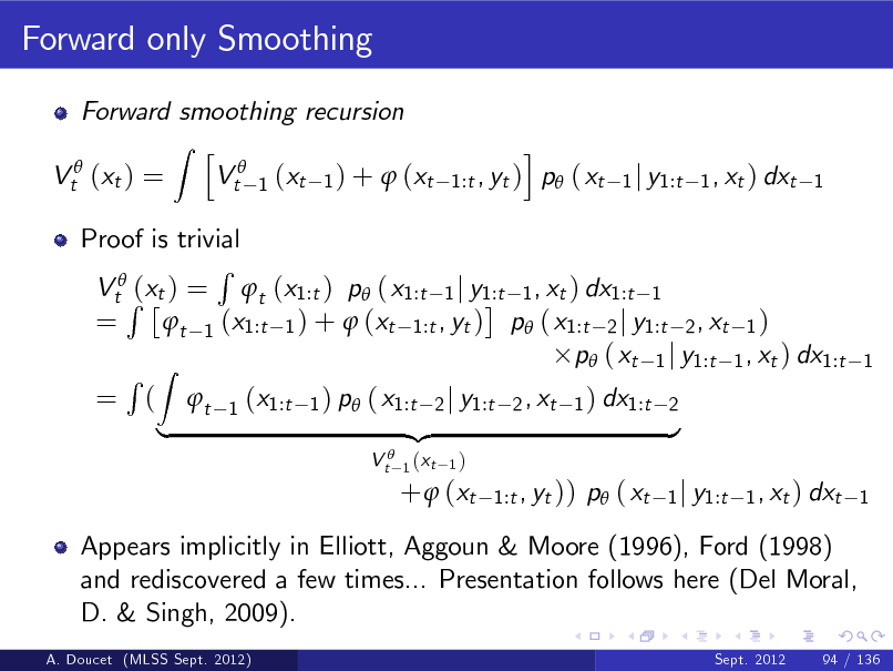
Forward only Smoothing
Forward smoothing recursion Z h Vt 1 (xt 1 ) + (xt Vt (xt ) = i , yt ) p ( xt 1:t
1 j y1:t 1 , xt ) dxt 1
Proof is trivial R VtR(xt ) = t (x1:t ) p ( x1:t 1 j y1:t 1 , xt ) dx1:t 1 = t 1 (x1:t 1 ) + (xt 1:t , yt ) p ( x1:t 2 j y1:t 2 , xt 1 ) p ( xt 1 j y1:t 1 , xt ) dx1:t R Z = ( t 1 (x1:t 1 ) p ( x1:t 2 j y1:t 2 , xt 1 ) dx1:t 2 {z } |
V t 1 (xt
1)
1
+ (xt
1:t , yt ))
p ( xt
1 j y1:t 1 , xt ) dxt 1
Appears implicitly in Elliott, Aggoun & Moore (1996), Ford (1998) and rediscovered a few times... Presentation follows here (Del Moral, D. & Singh, 2009).
A. Doucet (MLSS Sept. 2012) Sept. 2012 94 / 136
285
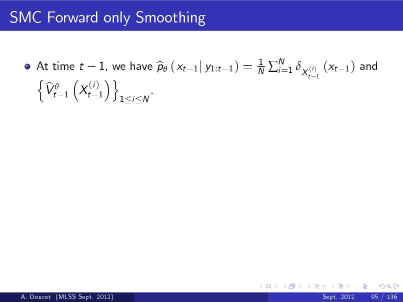
SMC Forward only Smoothing
At time t 1, we have p ( xt b n o (i ) b Vt 1 Xt 1 .
1 i N 1 j y1:t 1 )
=
1 N
N 1 X (i ) (xt i=
t 1
1)
and
A. Doucet (MLSS Sept. 2012)
Sept. 2012
95 / 136
286
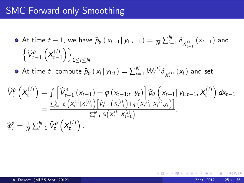
SMC Forward only Smoothing
At time t 1, we have p ( xt b n o (i ) b Vt 1 Xt 1 .
1 i N 1 j y1:t 1 )
=
1 N
N 1 X (i ) (xt i=
t 1
1)
and
(i ) b Vt Xt =
At time t, compute p ( xt j y1:t ) = N 1 Wt X (i ) (xt ) and set b i=
t
(i )
=
Rh
N 1 f j=
b Vt
bt =
1 N
(i ) b . N 1 Vt Xt i=
(i ) b 1 ) + (xt 1:t , yt ) p xt 1 j y1:t 1 , Xt h i (i ) (j ) (j ) (j ) (i ) b X t jX t 1 V t 1 X t 1 + X t 1 ,X t ,yt
1
(xt
i
dxt
1
N 1 f X t jX t j=
(i )
(j ) 1
,
A. Doucet (MLSS Sept. 2012)
Sept. 2012
95 / 136
287
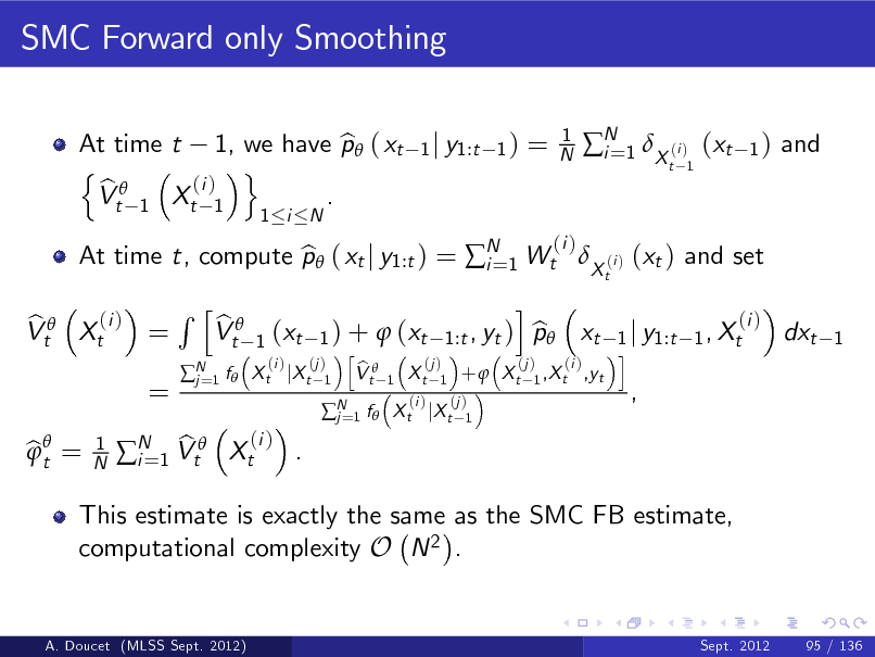
SMC Forward only Smoothing
At time t 1, we have p ( xt b n o (i ) b Vt 1 Xt 1 .
1 i N 1 j y1:t 1 )
=
1 N
N 1 X (i ) (xt i=
t 1
1)
and
(i ) b Vt Xt =
At time t, compute p ( xt j y1:t ) = N 1 Wt X (i ) (xt ) and set b i=
t
(i )
=
Rh
N 1 f j=
b Vt
bt =
1 N
This estimate is exactly the same as the SMC FB estimate, computational complexity O N 2 .
Sept. 2012 95 / 136
(i ) b . N 1 Vt Xt i=
(i ) b 1 ) + (xt 1:t , yt ) p xt 1 j y1:t 1 , Xt h i (i ) (j ) (j ) (j ) (i ) b X t jX t 1 V t 1 X t 1 + X t 1 ,X t ,yt
1
(xt
i
dxt
1
N 1 f X t jX t j=
(i )
(j ) 1
,
A. Doucet (MLSS Sept. 2012)
288
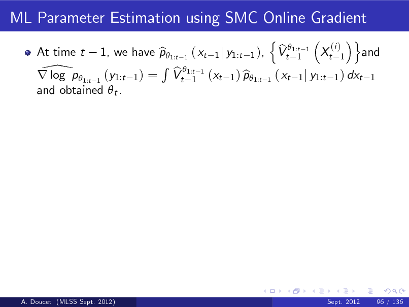
ML Parameter Estimation using SMC Online Gradient
At time t n o (i ) b 1, we have p 1:t 1 ( xt 1 j y1:t 1 ), Vt 1:t 1 Xt 1 and b 1 R 1:t 1 \p b r log 1:t 1 (y1:t 1 ) = Vt 1 (xt 1 ) p1:t 1 ( xt 1 j y1:t 1 ) dxt 1 b and obtained t .
A. Doucet (MLSS Sept. 2012)
Sept. 2012
96 / 136
289
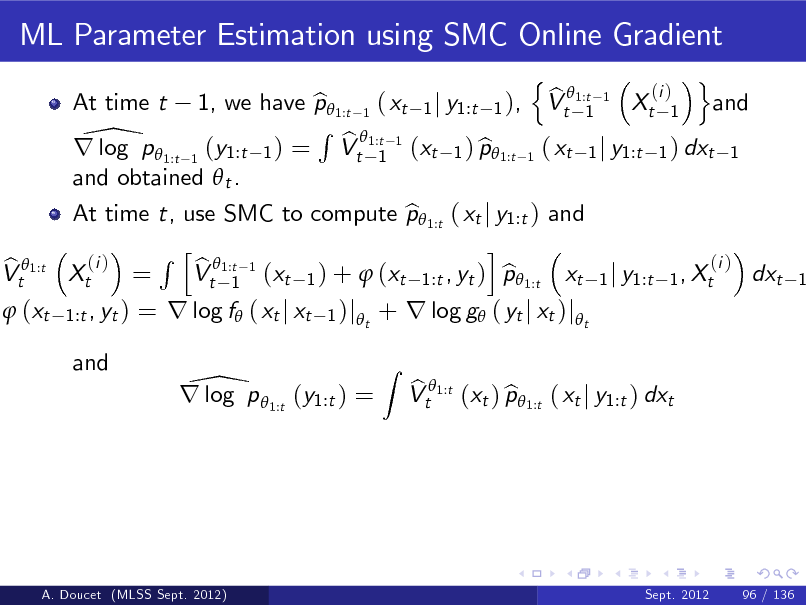
ML Parameter Estimation using SMC Online Gradient
n o (i ) b 1, we have p 1:t 1 ( xt 1 j y1:t 1 ), Vt 1:t 1 Xt 1 and b 1 R 1:t 1 \p b r log 1:t 1 (y1:t 1 ) = Vt 1 (xt 1 ) p1:t 1 ( xt 1 j y1:t 1 ) dxt 1 b and obtained t . At time t, use SMC to compute p 1:t ( xt j y1:t ) and b i R h 1:t 1 (i ) (i ) b Xt = Vt 1 (xt 1 ) + (xt 1:t , yt ) p 1:t xt 1 j y1:t 1 , Xt b dxt At time t
b Vt 1:t
1
(xt
1:t , yt )
= r log f ( xt j xt
1 )j t
+ r log g ( yt j xt )jt
Z
and
\ r log p 1:t (y1:t ) =
b b Vt 1:t (xt ) p 1:t ( xt j y1:t ) dxt
A. Doucet (MLSS Sept. 2012)
Sept. 2012
96 / 136
290
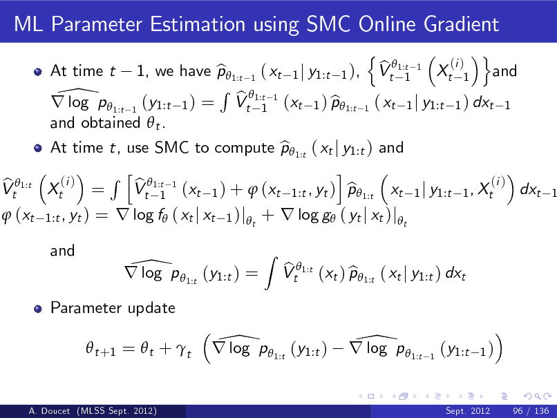
ML Parameter Estimation using SMC Online Gradient
n o (i ) b 1, we have p 1:t 1 ( xt 1 j y1:t 1 ), Vt 1:t 1 Xt 1 and b 1 R 1:t 1 \p b r log 1:t 1 (y1:t 1 ) = Vt 1 (xt 1 ) p1:t 1 ( xt 1 j y1:t 1 ) dxt 1 b and obtained t . At time t, use SMC to compute p 1:t ( xt j y1:t ) and b i R h 1:t 1 (i ) (i ) b Xt = Vt 1 (xt 1 ) + (xt 1:t , yt ) p 1:t xt 1 j y1:t 1 , Xt b dxt At time t
b Vt 1:t
1
(xt
1:t , yt )
= r log f ( xt j xt
1 )j t
+ r log g ( yt j xt )jt
Z
and
\ r log p 1:t (y1:t ) =
Parameter update t +1 = t + t
b b Vt 1:t (xt ) p 1:t ( xt j y1:t ) dxt
\ r log p 1:t (y1:t )
\ r log p 1:t
1
(y1:t
1)
A. Doucet (MLSS Sept. 2012)
Sept. 2012
96 / 136
291
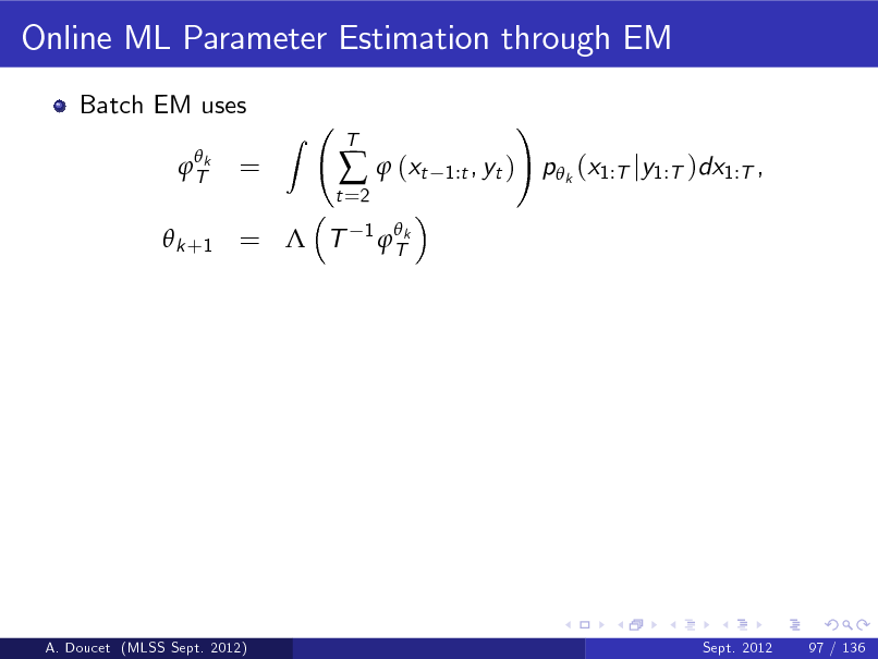
Online ML Parameter Estimation through EM
Batch EM uses
Tk
=
Z
t =2
(xt
1 Tk
T
1:t , yt )
!
p k (x1:T jy1:T )dx1:T ,
k +1 = T
A. Doucet (MLSS Sept. 2012)
Sept. 2012
97 / 136
292
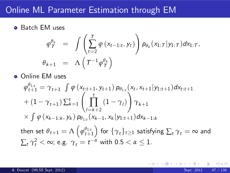
Online ML Parameter Estimation through EM
Batch EM uses
Tk
=
Z
t =2
(xt
1 Tk
T
1:t , yt )
!
p k (x1:T jy1:T )dx1:T ,
k +1 = T
Online EM uses R 1:t t +1 = t +1 (xt :t +1 , yt +1 ) p 1:t (xt , xt +1 jy1:t +1 )dxt :t +1 !
1:t then set t +1 = t +1
+ (1 R
t +1 ) t =1 k
l =k +2
t
(1
l )
k +1
(xk
1:k , yk ) p 1:t (xk 1 , xk jy1:t +1 )dxk 1:k
t 2 t
< ; e.g. t = t
with 0.5 <
for ft gt
1
satisfying t t = and 1.
A. Doucet (MLSS Sept. 2012)
Sept. 2012
97 / 136
293
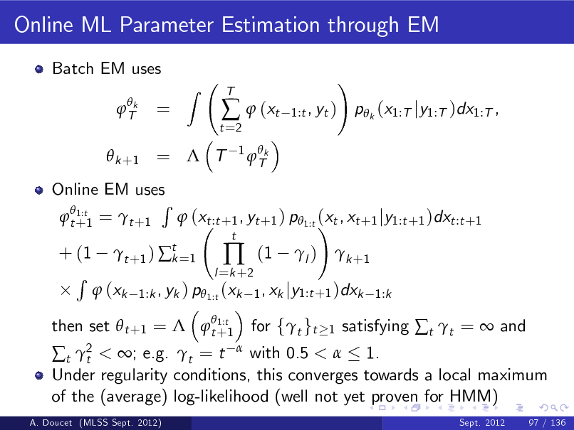
Online ML Parameter Estimation through EM
Batch EM uses
Tk
=
Z
t =2
(xt
1 Tk
T
1:t , yt )
!
p k (x1:T jy1:T )dx1:T ,
k +1 = T
Online EM uses R 1:t t +1 = t +1 (xt :t +1 , yt +1 ) p 1:t (xt , xt +1 jy1:t +1 )dxt :t +1 !
1:t then set t +1 = t +1
+ (1 R
t +1 ) t =1 k
l =k +2
t
(1
l )
k +1
(xk
1:k , yk ) p 1:t (xk 1 , xk jy1:t +1 )dxk 1:k
< ; e.g. t = t with 0.5 < 1. Under regularity conditions, this converges towards a local maximum of the (average) log-likelihood (well not yet proven for HMM)
t 2 t
A. Doucet (MLSS Sept. 2012) Sept. 2012 97 / 136
for ft gt
1
satisfying t t = and
294
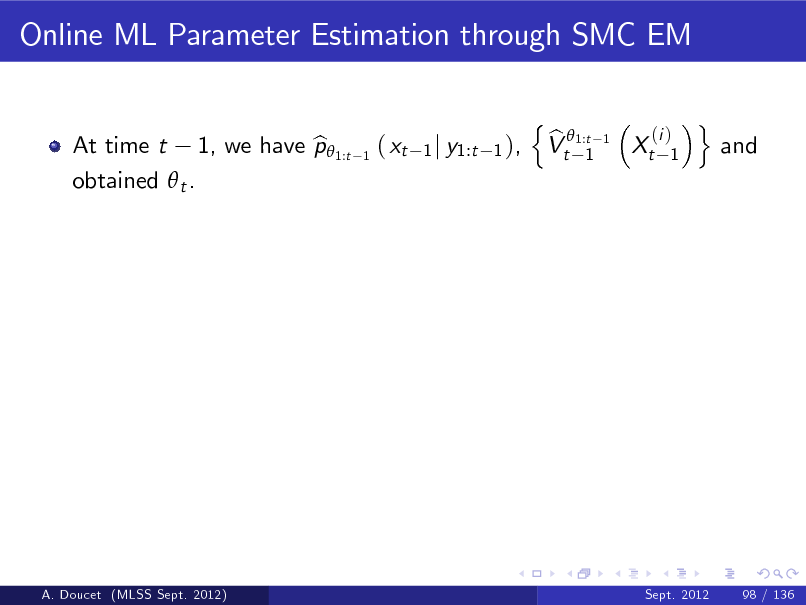
Online ML Parameter Estimation through SMC EM
n b Vt 1:t 1
(i ) 1
At time t 1, we have p 1:t b obtained t .
1
( xt
1 j y1:t 1 ),
1
Xt
o
and
A. Doucet (MLSS Sept. 2012)
Sept. 2012
98 / 136
295
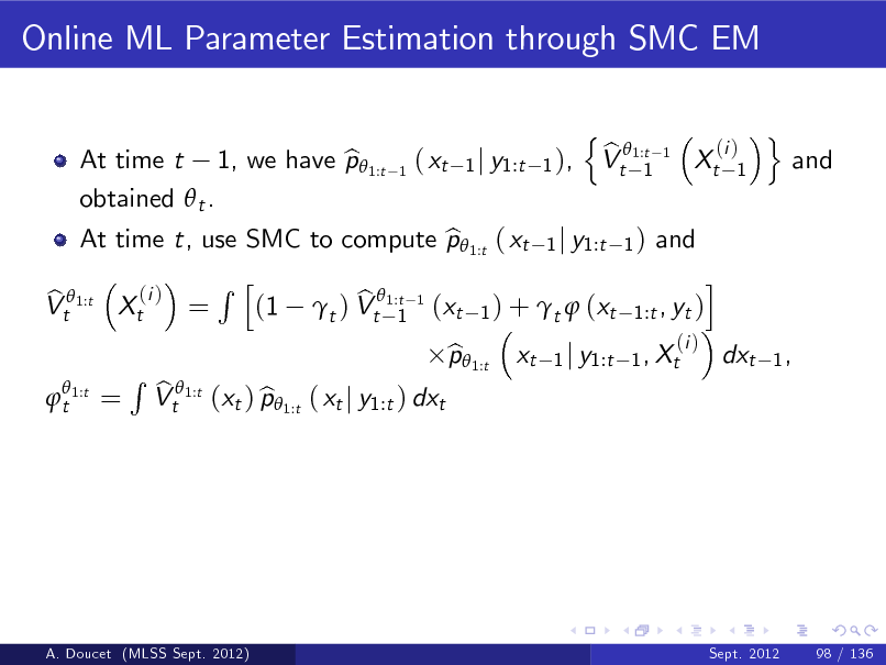
Online ML Parameter Estimation through SMC EM
n b Vt 1:t 1
(i ) 1
At time t, use SMC to compute p 1:t ( xt 1 j y1:t 1 ) and b i Rh (i ) b b Vt 1:t Xt = (1 t ) Vt1:t 1 (xt 1 ) + t (xt 1:t , yt ) 1
t 1:t
At time t 1, we have p 1:t b obtained t .
1
( xt
1 j y1:t 1 ),
1
Xt
o
and
=
R
b Vt 1:t (xt ) p 1:t ( xt j y1:t ) dxt b
p 1:t b
xt
(i ) 1 j y1:t 1 , Xt
dxt
1,
A. Doucet (MLSS Sept. 2012)
Sept. 2012
98 / 136
296
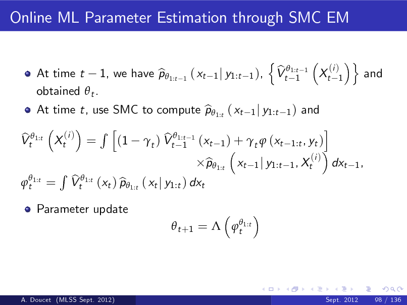
Online ML Parameter Estimation through SMC EM
n b Vt 1:t 1
(i ) 1
At time t, use SMC to compute p 1:t ( xt 1 j y1:t 1 ) and b i Rh (i ) b b Vt 1:t Xt = (1 t ) Vt1:t 1 (xt 1 ) + t (xt 1:t , yt ) 1
t 1:t
At time t 1, we have p 1:t b obtained t .
1
( xt
1 j y1:t 1 ),
1
Xt
o
and
=
Parameter update
R
b Vt 1:t (xt ) p 1:t ( xt j y1:t ) dxt b
p 1:t b
xt
(i ) 1 j y1:t 1 , Xt
dxt
1,
t +1 = t 1:t
A. Doucet (MLSS Sept. 2012)
Sept. 2012
98 / 136
297
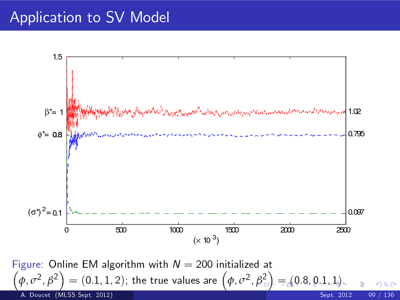
Application to SV Model
1.5
*= 1 *= 0.8
1.02 0.795
(*) 2= 0.1 0 500 1000 ( 10 3) 1500 2000
0.097 2500
Figure: Online EM algorithm with N = 200 initialized at , 2 , 2 = (0.1, 1, 2); the true values are , 2 , 2 = (0.8, 0.1, 1).
A. Doucet (MLSS Sept. 2012) Sept. 2012 99 / 136
298
Direct SMC vs Forward Smoothing for Online EM
For online gradient techniques, forward smoothing is stable contrary to the direct method.
A. Doucet (MLSS Sept. 2012)
Sept. 2012
100 / 136
299
Direct SMC vs Forward Smoothing for Online EM
For online gradient techniques, forward smoothing is stable contrary to the direct method. Structure of online EM is signicantly dierent.
A. Doucet (MLSS Sept. 2012)
Sept. 2012
100 / 136
300
Direct SMC vs Forward Smoothing for Online EM
For online gradient techniques, forward smoothing is stable contrary to the direct method. Structure of online EM is signicantly dierent. We have seen previously that the MSE for smoothed additive functionals is of the same order for direct and FB estimates.
A. Doucet (MLSS Sept. 2012)
Sept. 2012
100 / 136
301
Direct SMC vs Forward Smoothing for Online EM
For online gradient techniques, forward smoothing is stable contrary to the direct method. Structure of online EM is signicantly dierent. We have seen previously that the MSE for smoothed additive functionals is of the same order for direct and FB estimates. Direct method is variance dominated, FB is bias dominated.
A. Doucet (MLSS Sept. 2012)
Sept. 2012
100 / 136
302
Direct SMC vs Forward Smoothing for Online EM
For online gradient techniques, forward smoothing is stable contrary to the direct method. Structure of online EM is signicantly dierent. We have seen previously that the MSE for smoothed additive functionals is of the same order for direct and FB estimates. Direct method is variance dominated, FB is bias dominated. We compare experimentally both methods on a simple linear Gaussian model over 100 runs.
A. Doucet (MLSS Sept. 2012)
Sept. 2012
100 / 136
303
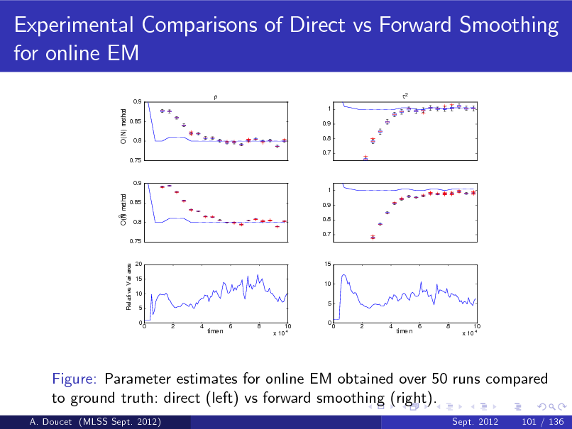
Experimental Comparisons of Direct vs Forward Smoothing for online EM
0.9
O(N) method
1
2
0.85 0.8 0.75
0.9 0.8 0.7
0.9
O(N met hod )
1 0.85 0.8 0.75 0.9 0.8 0.7
2
Rel at i ve Vari ance
20 15 10 5 0 0 2 4 6 8 10 x 10 4
15 10 5 0
time n
0
2
4
time n
6
8
10 x 10 4
Figure: Parameter estimates for online EM obtained over 50 runs compared to ground truth: direct (left) vs forward smoothing (right).
A. Doucet (MLSS Sept. 2012) Sept. 2012 101 / 136
304
Summary
SMC smoothing techniques can be used to perform o-line and on-line ML parameter estimation.
A. Doucet (MLSS Sept. 2012)
Sept. 2012
102 / 136
305
Summary
SMC smoothing techniques can be used to perform o-line and on-line ML parameter estimation. FB estimates for smoothed additive functionals can be computed using a forward only procedure.
A. Doucet (MLSS Sept. 2012)
Sept. 2012
102 / 136
306
Summary
SMC smoothing techniques can be used to perform o-line and on-line ML parameter estimation. FB estimates for smoothed additive functionals can be computed using a forward only procedure. Forward smoothing allows us to implement a degeneracy free on-line gradient ascent algorithm.
A. Doucet (MLSS Sept. 2012)
Sept. 2012
102 / 136
307
Summary
SMC smoothing techniques can be used to perform o-line and on-line ML parameter estimation. FB estimates for smoothed additive functionals can be computed using a forward only procedure. Forward smoothing allows us to implement a degeneracy free on-line gradient ascent algorithm. For on-line EM, forward smoothing and direct methods have both pros and cons with no clear winner.
A. Doucet (MLSS Sept. 2012)
Sept. 2012
102 / 136
308
Summary
SMC smoothing techniques can be used to perform o-line and on-line ML parameter estimation. FB estimates for smoothed additive functionals can be computed using a forward only procedure. Forward smoothing allows us to implement a degeneracy free on-line gradient ascent algorithm. For on-line EM, forward smoothing and direct methods have both pros and cons with no clear winner. Bias reduction approaches are currently under study.
A. Doucet (MLSS Sept. 2012)
Sept. 2012
102 / 136
309

Bayesian Parameter Inference in State-Space Models
Assume we have Xt j (Xt
= xt 1 ) Yt j (Xt = xt )
1
f ( xt j xt
1) ,
g ( yt j xt ) ,
where is an unknown static parameter with prior p ( ).
A. Doucet (MLSS Sept. 2012)
Sept. 2012
103 / 136
310
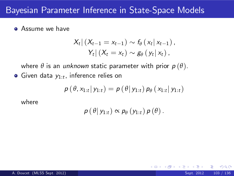
Bayesian Parameter Inference in State-Space Models
Assume we have Xt j (Xt
= xt 1 ) Yt j (Xt = xt )
1
f ( xt j xt
1) ,
g ( yt j xt ) ,
where is an unknown static parameter with prior p ( ). Given data y1:t , inference relies on p ( , x1:t j y1:t ) = p ( j y1:t ) p ( x1:t j y1:t ) where p ( j y1:t ) p (y1:t ) p ( ) .
A. Doucet (MLSS Sept. 2012)
Sept. 2012
103 / 136
311
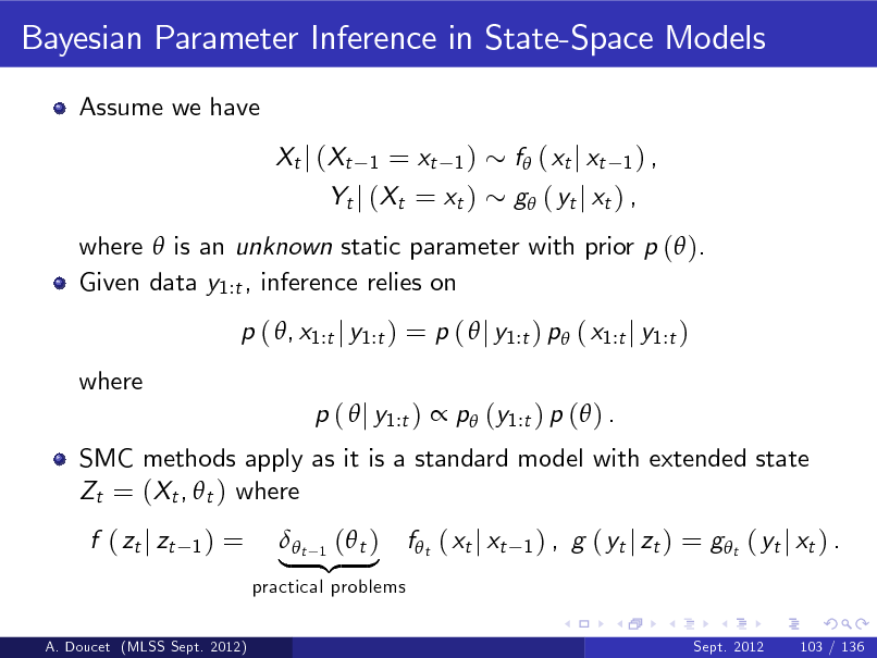
Bayesian Parameter Inference in State-Space Models
Assume we have Xt j (Xt
= xt 1 ) Yt j (Xt = xt )
1
f ( xt j xt
1) ,
g ( yt j xt ) ,
where is an unknown static parameter with prior p ( ). Given data y1:t , inference relies on p ( , x1:t j y1:t ) = p ( j y1:t ) p ( x1:t j y1:t ) where SMC methods apply as it is a standard model with extended state Zt = (Xt , t ) where f ( zt j zt
1)
p ( j y1:t ) p (y1:t ) p ( ) .
=
practical problems
A. Doucet (MLSS Sept. 2012) Sept. 2012 103 / 136
1 ( t ) | t {z }
f t ( xt j xt
1) ,
g ( yt j zt ) = g t ( yt j xt ) .
312
![Slide: Cautionary Warning
2 For xed , V [p (y1:t )] /p (y1:t ) is in O (t/N ). b
A. Doucet (MLSS Sept. 2012)
Sept. 2012
104 / 136](https://yosinski.com/mlss12/media/slides/MLSS-2012-Doucet-Sequential-Monte-Carlo-Methods_313.png)
Cautionary Warning
2 For xed , V [p (y1:t )] /p (y1:t ) is in O (t/N ). b
A. Doucet (MLSS Sept. 2012)
Sept. 2012
104 / 136
313
![Slide: Cautionary Warning
2 For xed , V [p (y1:t )] /p (y1:t ) is in O (t/N ). b
In a Bayesian context, the problem is even more complex as p ( j y1:t ) p (y1:t ) p ( ) and we have t = for all t so the latent process does not enjoy mixing properties.
A. Doucet (MLSS Sept. 2012)
Sept. 2012
104 / 136](https://yosinski.com/mlss12/media/slides/MLSS-2012-Doucet-Sequential-Monte-Carlo-Methods_314.png)
Cautionary Warning
2 For xed , V [p (y1:t )] /p (y1:t ) is in O (t/N ). b
In a Bayesian context, the problem is even more complex as p ( j y1:t ) p (y1:t ) p ( ) and we have t = for all t so the latent process does not enjoy mixing properties.
A. Doucet (MLSS Sept. 2012)
Sept. 2012
104 / 136
314
![Slide: Cautionary Warning
2 For xed , V [p (y1:t )] /p (y1:t ) is in O (t/N ). b
In a Bayesian context, the problem is even more complex as p ( j y1:t ) p (y1:t ) p ( ) and we have t = for all t so the latent process does not enjoy mixing properties. A seemingly attractive idea consists of using MCMC steps on ; e.g. (Andrieu, De Freitas & D.,1999; Fearnhead, 2002; Gilks & Berzuini 2001; Storvik, 2002; Carvalho et al., 2010) so as to introduce some noise on the component of the state.
A. Doucet (MLSS Sept. 2012)
Sept. 2012
104 / 136](https://yosinski.com/mlss12/media/slides/MLSS-2012-Doucet-Sequential-Monte-Carlo-Methods_315.png)
Cautionary Warning
2 For xed , V [p (y1:t )] /p (y1:t ) is in O (t/N ). b
In a Bayesian context, the problem is even more complex as p ( j y1:t ) p (y1:t ) p ( ) and we have t = for all t so the latent process does not enjoy mixing properties. A seemingly attractive idea consists of using MCMC steps on ; e.g. (Andrieu, De Freitas & D.,1999; Fearnhead, 2002; Gilks & Berzuini 2001; Storvik, 2002; Carvalho et al., 2010) so as to introduce some noise on the component of the state.
A. Doucet (MLSS Sept. 2012)
Sept. 2012
104 / 136
315
![Slide: Cautionary Warning
2 For xed , V [p (y1:t )] /p (y1:t ) is in O (t/N ). b
In a Bayesian context, the problem is even more complex as p ( j y1:t ) p (y1:t ) p ( ) and we have t = for all t so the latent process does not enjoy mixing properties. A seemingly attractive idea consists of using MCMC steps on ; e.g. (Andrieu, De Freitas & D.,1999; Fearnhead, 2002; Gilks & Berzuini 2001; Storvik, 2002; Carvalho et al., 2010) so as to introduce some noise on the component of the state. When p ( j y1:t , x1:t ) = p ( j st (x1:t , y1:t )) where st (x1:t , y1:t ) is a xed-dimensional of su cient statistics, the algorithm is particularly elegant but still implicitly relies on SMC approximation of p ( x1:t j y1:t ) so degeneracy will creep in.
A. Doucet (MLSS Sept. 2012)
Sept. 2012
104 / 136](https://yosinski.com/mlss12/media/slides/MLSS-2012-Doucet-Sequential-Monte-Carlo-Methods_316.png)
Cautionary Warning
2 For xed , V [p (y1:t )] /p (y1:t ) is in O (t/N ). b
In a Bayesian context, the problem is even more complex as p ( j y1:t ) p (y1:t ) p ( ) and we have t = for all t so the latent process does not enjoy mixing properties. A seemingly attractive idea consists of using MCMC steps on ; e.g. (Andrieu, De Freitas & D.,1999; Fearnhead, 2002; Gilks & Berzuini 2001; Storvik, 2002; Carvalho et al., 2010) so as to introduce some noise on the component of the state. When p ( j y1:t , x1:t ) = p ( j st (x1:t , y1:t )) where st (x1:t , y1:t ) is a xed-dimensional of su cient statistics, the algorithm is particularly elegant but still implicitly relies on SMC approximation of p ( x1:t j y1:t ) so degeneracy will creep in.
A. Doucet (MLSS Sept. 2012)
Sept. 2012
104 / 136
316
![Slide: Cautionary Warning
2 For xed , V [p (y1:t )] /p (y1:t ) is in O (t/N ). b
In a Bayesian context, the problem is even more complex as p ( j y1:t ) p (y1:t ) p ( ) and we have t = for all t so the latent process does not enjoy mixing properties. A seemingly attractive idea consists of using MCMC steps on ; e.g. (Andrieu, De Freitas & D.,1999; Fearnhead, 2002; Gilks & Berzuini 2001; Storvik, 2002; Carvalho et al., 2010) so as to introduce some noise on the component of the state. When p ( j y1:t , x1:t ) = p ( j st (x1:t , y1:t )) where st (x1:t , y1:t ) is a xed-dimensional of su cient statistics, the algorithm is particularly elegant but still implicitly relies on SMC approximation of p ( x1:t j y1:t ) so degeneracy will creep in. As dim (Zt ) = dim (Xt ) + dim ( ), such methods are not recommended for high-dimensional , especially with vague priors.
Sept. 2012
A. Doucet (MLSS Sept. 2012)
104 / 136](https://yosinski.com/mlss12/media/slides/MLSS-2012-Doucet-Sequential-Monte-Carlo-Methods_317.png)
Cautionary Warning
2 For xed , V [p (y1:t )] /p (y1:t ) is in O (t/N ). b
In a Bayesian context, the problem is even more complex as p ( j y1:t ) p (y1:t ) p ( ) and we have t = for all t so the latent process does not enjoy mixing properties. A seemingly attractive idea consists of using MCMC steps on ; e.g. (Andrieu, De Freitas & D.,1999; Fearnhead, 2002; Gilks & Berzuini 2001; Storvik, 2002; Carvalho et al., 2010) so as to introduce some noise on the component of the state. When p ( j y1:t , x1:t ) = p ( j st (x1:t , y1:t )) where st (x1:t , y1:t ) is a xed-dimensional of su cient statistics, the algorithm is particularly elegant but still implicitly relies on SMC approximation of p ( x1:t j y1:t ) so degeneracy will creep in. As dim (Zt ) = dim (Xt ) + dim ( ), such methods are not recommended for high-dimensional , especially with vague priors.
Sept. 2012
A. Doucet (MLSS Sept. 2012)
104 / 136
317
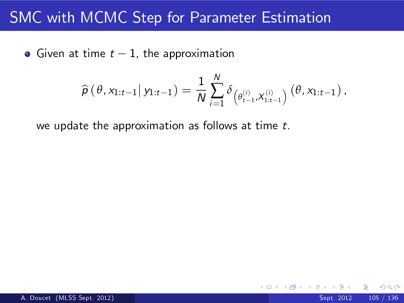
SMC with MCMC Step for Parameter Estimation
Given at time t p ( , x1:t b 1, the approximation
1 j y1:t 1 )
=
1 N
i =1
N
t
(i )
(i ) 1 ,X 1:t 1
(, x1:t
1) ,
we update the approximation as follows at time t.
A. Doucet (MLSS Sept. 2012)
Sept. 2012
105 / 136
318
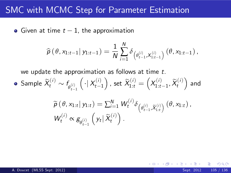
SMC with MCMC Step for Parameter Estimation
Given at time t p ( , x1:t b 1, the approximation
1 j y1:t 1 )
=
1 N
i =1
N
t
(i )
(i ) 1 ,X 1:t 1
(, x1:t
1) ,
we update the approximation as follows at time t. (i ) (i ) e ( i ) f (i ) e (i ) e (i ) Sample Xt j Xt 1 , set X1:t = X1:t 1 , Xt
t 1
and
Wt
p ( , x1:t j y1:t ) = N 1 Wt e i=
(i )
(i )
t
(i )
g (i )
t 1
e (i ) . yt j Xt
e (i ) 1 ,X 1:t
(, x1:t ) ,
A. Doucet (MLSS Sept. 2012)
Sept. 2012
105 / 136
319
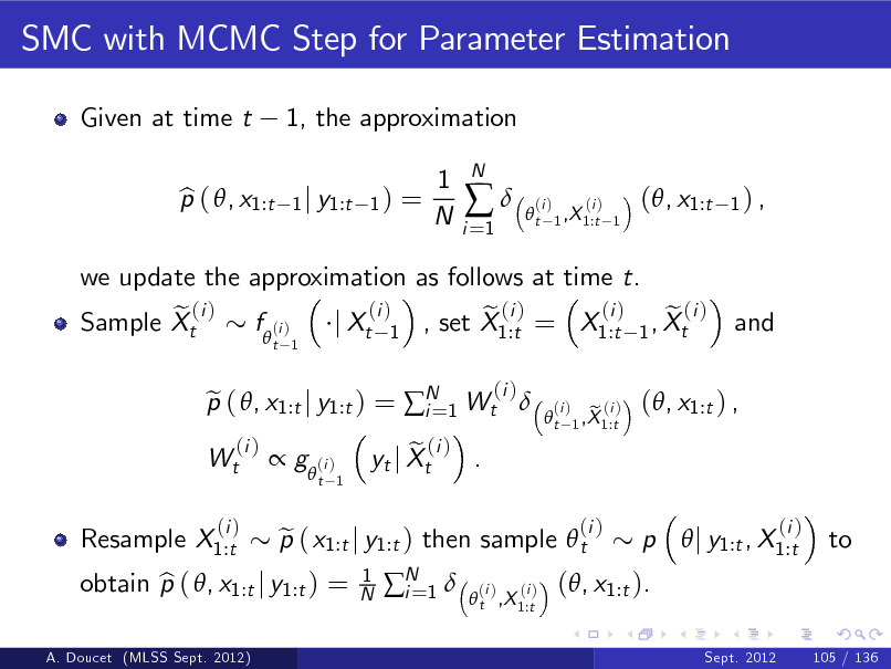
SMC with MCMC Step for Parameter Estimation
Given at time t p ( , x1:t b 1, the approximation
1 j y1:t 1 )
=
1 N
i =1
N
t
(i )
(i ) 1 ,X 1:t 1
(, x1:t
1) ,
we update the approximation as follows at time t. (i ) (i ) e ( i ) f (i ) e (i ) e (i ) Sample Xt j Xt 1 , set X1:t = X1:t 1 , Xt
t 1
and
Wt Resample X1:t
p ( , x1:t j y1:t ) = N 1 Wt e i=
(i )
(i )
t
(i )
g (i )
t 1
(i )
A. Doucet (MLSS Sept. 2012)
obtain p ( , x1:t j y1:t ) = b
p ( x1:t j y1:t ) then sample t e
1 N
e (i ) . yt j Xt N 1 i=
e (i ) 1 ,X 1:t
(, x1:t ) ,
(i )
t ,X 1:t
(i )
(i )
(, x1:t ).
p j y1:t , X1:t
(i )
to
Sept. 2012
105 / 136
320
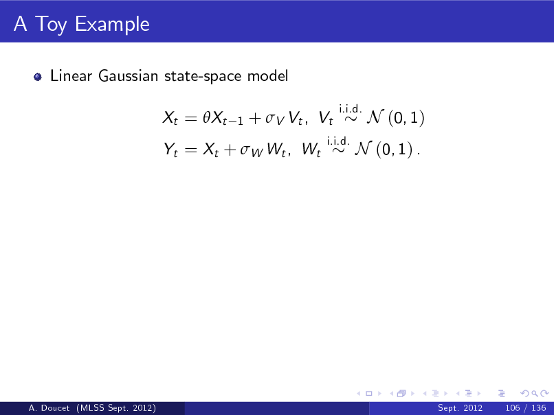
A Toy Example
Linear Gaussian state-space model Xt = Xt
1
+ V Vt , Vt
i.i.d.
Yt = Xt + W Wt , Wt
i.i.d.
N (0, 1)
N (0, 1) .
A. Doucet (MLSS Sept. 2012)
Sept. 2012
106 / 136
321
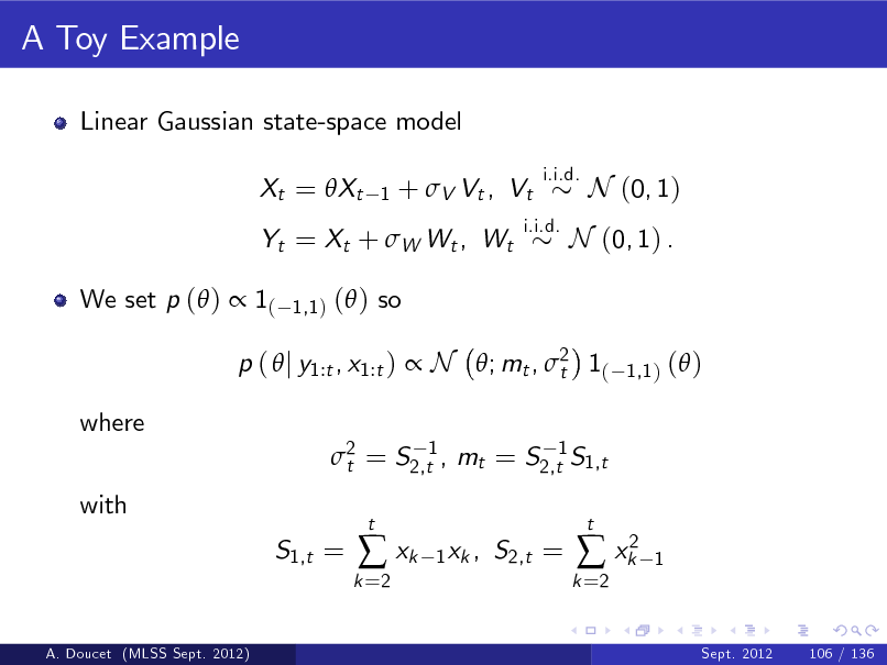
A Toy Example
Linear Gaussian state-space model Xt = Xt
1
+ V Vt , Vt
i.i.d.
Yt = Xt + W Wt , Wt We set p ( ) 1(
1,1 )
i.i.d.
N (0, 1)
N (0, 1) .
( ) so
1,1 )
p ( j y1:t , x1:t ) N ; mt , 2 1( t where 2 = S2,t1 , mt = S2,t1 S1,t t with S1,t =
( )
k =2
xk
t
1 xk ,
S2,t =
k =2
xk2
t
1
A. Doucet (MLSS Sept. 2012)
Sept. 2012
106 / 136
322
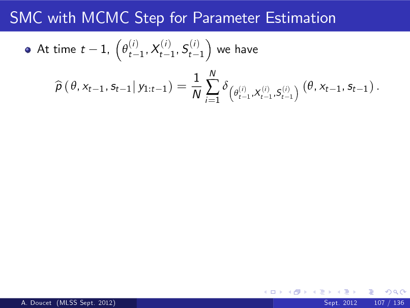
SMC with MCMC Step for Parameter Estimation
At time t p ( , xt b 1, t
1 , st
(i )
(i ) (i ) 1 , Xt 1 , St 1
1) =
we have
1 j y1:t
1 N
i =1
N
t
(i )
(i ) (i ) 1 ,X t 1 ,S t 1
(, xt
1 , st 1 ) .
A. Doucet (MLSS Sept. 2012)
Sept. 2012
107 / 136
323
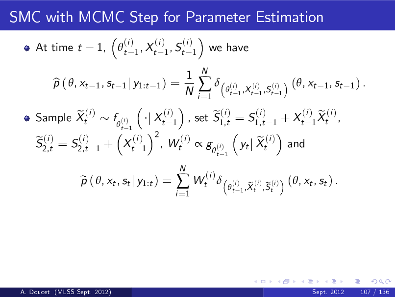
SMC with MCMC Step for Parameter Estimation
At time t p ( , xt b 1, t
1 , st
(i )
(i ) (i ) 1 , Xt 1 , St 1
1) =
we have
1 j y1:t
1 N
i =1
N
t
(i )
(i ) (i ) 1 ,X t 1 ,S t 1
(, xt
1 , st 1 ) .
e (i ) Sample Xt
(i ) e (i ) S2,t = S2,t
f (i )
1
t 1
+ Xt
(i ) 2 , 1
j Xt
(i ) 1
Wt
(i )
(i ) e (i ) , set S1,t = S1,t
1
+ Xt
g (i )
(i )
t 1
p ( , xt , st j y1:t ) = e
i =1
Wt
N
e yt j Xt
(i )
and
(i ) e (i ) 1 Xt ,
t
(i )
e (i ) e (i ) 1 ,X t ,S t
(, xt , st ) .
A. Doucet (MLSS Sept. 2012)
Sept. 2012
107 / 136
324
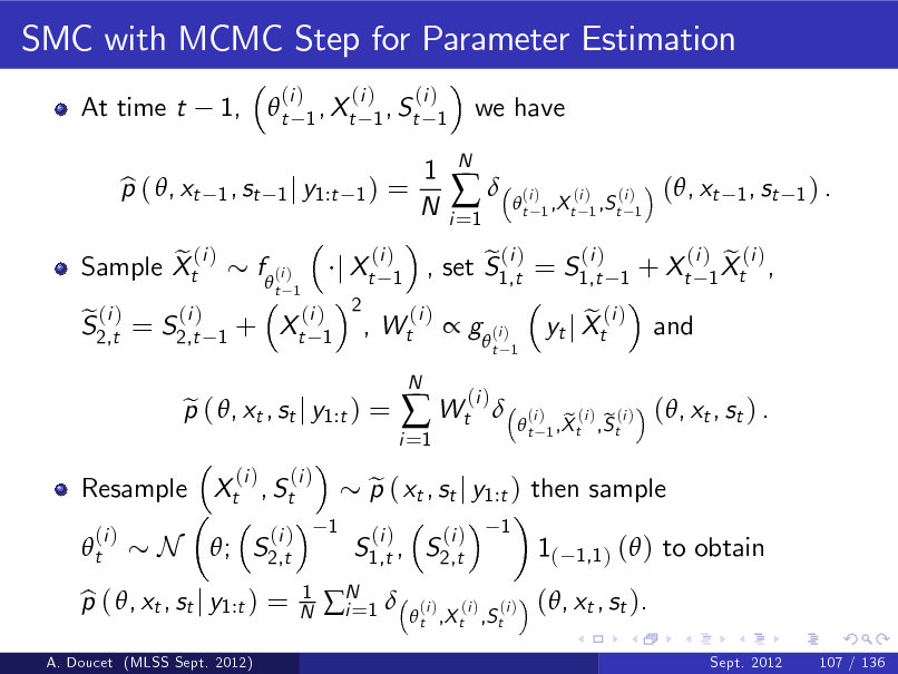
SMC with MCMC Step for Parameter Estimation
At time t p ( , xt b 1, t
1 , st
(i )
(i ) (i ) 1 , Xt 1 , St 1
1) =
we have
1 j y1:t
1 N
i =1
N
t
(i )
(i ) (i ) 1 ,X t 1 ,S t 1
(, xt
1 , st 1 ) .
e (i ) Sample Xt
(i ) e (i ) S2,t = S2,t
f (i )
1
t 1
+ Xt
(i ) 2 , 1
j Xt
(i ) 1
Wt
(i )
(i ) e (i ) , set S1,t = S1,t
1
+ Xt
g (i )
(i )
t 1
Resample Xt , St t
(i )
p ( , xt , st j y1:t ) = e
(i ) (i )
i =1
Wt
(i )
N
e yt j Xt
(i )
and
(i ) e (i ) 1 Xt ,
t
(i )
N
; S2,t
(i )
1 N
1
S1,t , S2,t
(i )
p ( xt , st j y1:t ) then sample e
(i )
1
e (i ) e (i ) 1 ,X t ,S t
(, xt , st ) .
1(
1,1 )
( ) to obtain
A. Doucet (MLSS Sept. 2012)
p ( , xt , st j y1:t ) = b
N 1 i=
t ,X t ,S t
(i )
(i )
(, xt , st ).
Sept. 2012 107 / 136
325
![Slide: Illustration of the Degeneracy Problem
0 .7 0 .6 0 .5 0 .4 0 .3 0 .2 0 .1 0
0
50 0
10 00
10 50
20 00
20 50
30 00
30 50
40 00
40 50
50 00
SMC estimate of E [ j y1:t ], as t increases the degeneracy creeps in.
A. Doucet (MLSS Sept. 2012) Sept. 2012 108 / 136](https://yosinski.com/mlss12/media/slides/MLSS-2012-Doucet-Sequential-Monte-Carlo-Methods_326.png)
Illustration of the Degeneracy Problem
0 .7 0 .6 0 .5 0 .4 0 .3 0 .2 0 .1 0
0
50 0
10 00
10 50
20 00
20 50
30 00
30 50
40 00
40 50
50 00
SMC estimate of E [ j y1:t ], as t increases the degeneracy creeps in.
A. Doucet (MLSS Sept. 2012) Sept. 2012 108 / 136
326
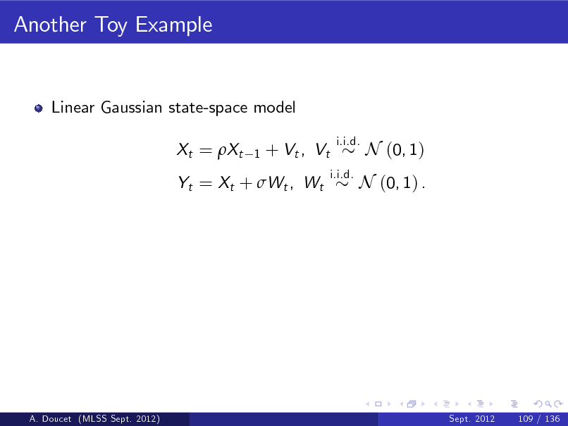
Another Toy Example
Linear Gaussian state-space model Xt = Xt
1
+ Vt , Vt
i.i.d. i.i.d.
N (0, 1)
Yt = Xt + Wt , Wt
N (0, 1) .
A. Doucet (MLSS Sept. 2012)
Sept. 2012
109 / 136
327
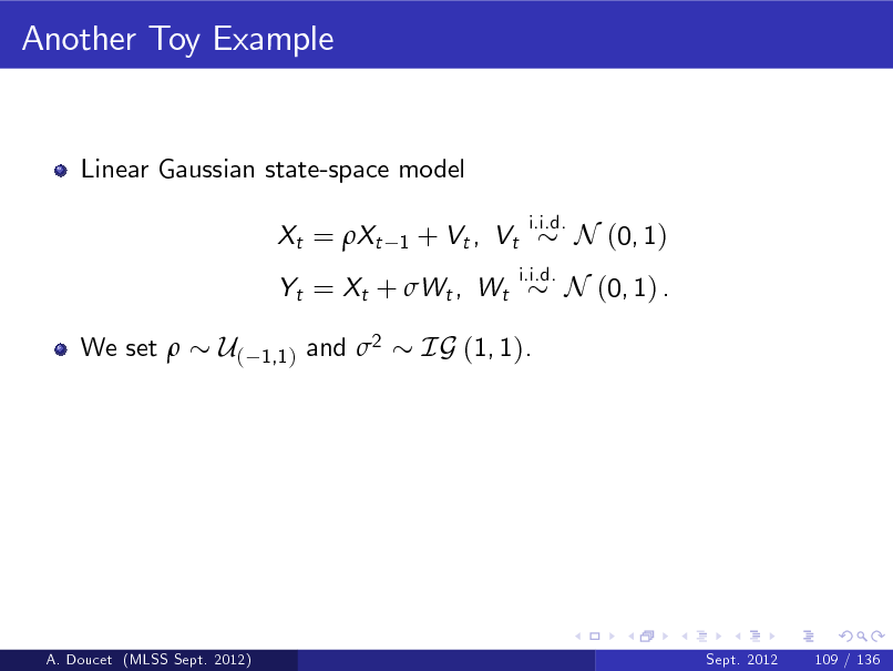
Another Toy Example
Linear Gaussian state-space model Xt = Xt
1
+ Vt , Vt
i.i.d. i.i.d.
N (0, 1)
Yt = Xt + Wt , Wt We set
N (0, 1) .
U(
1,1 )
and 2
IG (1, 1).
A. Doucet (MLSS Sept. 2012)
Sept. 2012
109 / 136
328
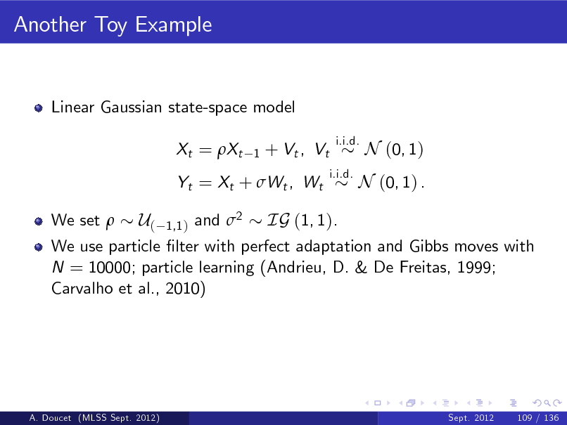
Another Toy Example
Linear Gaussian state-space model Xt = Xt
1
+ Vt , Vt
i.i.d. i.i.d.
N (0, 1)
Yt = Xt + Wt , Wt We set
N (0, 1) .
U( 1,1 ) and 2 IG (1, 1). We use particle lter with perfect adaptation and Gibbs moves with N = 10000; particle learning (Andrieu, D. & De Freitas, 1999; Carvalho et al., 2010)
A. Doucet (MLSS Sept. 2012)
Sept. 2012
109 / 136
329
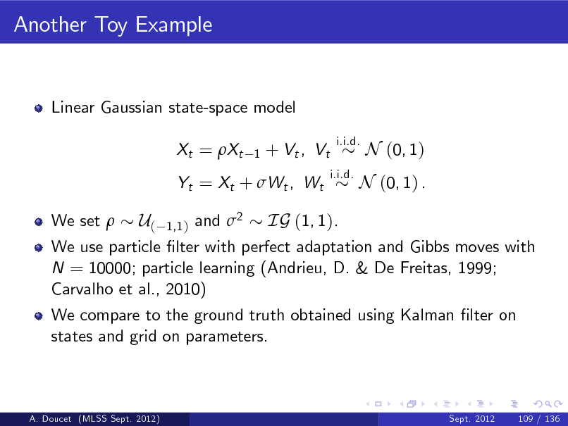
Another Toy Example
Linear Gaussian state-space model Xt = Xt
1
+ Vt , Vt
i.i.d. i.i.d.
N (0, 1)
Yt = Xt + Wt , Wt We set
N (0, 1) .
U( 1,1 ) and 2 IG (1, 1). We use particle lter with perfect adaptation and Gibbs moves with N = 10000; particle learning (Andrieu, D. & De Freitas, 1999; Carvalho et al., 2010) We compare to the ground truth obtained using Kalman lter on states and grid on parameters.
A. Doucet (MLSS Sept. 2012)
Sept. 2012
109 / 136
330
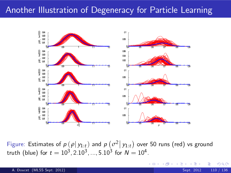
Another Illustration of Degeneracy for Particle Learning
pdf , n=1000
04 .0 03 .0 02 .0 01 .0 0.8 0 0 .9 1 1 .1 1 .2 04 .0 03 .0 02 .0 01 .0 0.8 0 0 .9 1 1 .1 1 .2 04 .0 03 .0 02 .0 01 .0 0.8 0 0 .9 1 1 .1 1 .2 04 .0 03 .0 02 .0 01 .0 0.8 0 0 .9 1 1 .1 1 .2 04 .0 03 .0 02 .0 01 .0 0.8 0 0 .9 1 2 y 1 .1 1 .2
0 .1 05 .0 0.4 0 06 .0 04 .0 02 .0 0.4 0 0 .1 05 .0 0.4 0 0 .1 05 .0 0.4 0 0 .1 05 .0 0.4 0 0 .5 0 .6 0 .7 0 .8 0 .9 0 .5 0 .6 0 .7 0 .8 0 .9 0 .5 0 .6 0 .7 0 .8 0 .9 0 .5 0 .6 0 .7 0 .8 0 .9 0 .5 0 .6 0 .7 0 .8 0 .9
pdf , n=5000
pdf , n=4000
pdf , n=3000
pdf , n=2000
Figure: Estimates of p ( j y1 :t ) and p 2 y1 :t over 50 runs (red) vs ground truth (blue) for t = 103 , 2.103 , ..., 5.103 for N = 104 .
A. Doucet (MLSS Sept. 2012) Sept. 2012 110 / 136
331
Online Bayesian Parameter Estimation
All proposed procedures for online Bayesian parameter estimation are decient. Some articial dynamics can be introduced but then we do not approximate fp ( , x1:t j y1:t )gt 1 ; e.g. (Liu & West, 2001; Flury & Shephard, 2010). Methods based on MCMC steps are elegant but do suer from the degeneracy problem and provide unreliable approximations.
A. Doucet (MLSS Sept. 2012)
Sept. 2012
111 / 136
332
O- ine Bayesian Parameter Estimation
Given a collection of observations y1:T := (y1 , ..., yT ), T being xed, inference relies on the posterior density p ( , x1:T j y1:T ) = p ( j y1:T ) p ( x1:T j y1:T ) p (, x1:T , y1:T ) where p (, x1:T , y1:T ) p ( ) (x1 ) f ( xt j xt
t =2 T 1)
t =1
g ( yt j xt )
T
.
A. Doucet (MLSS Sept. 2012)
Sept. 2012
112 / 136
333
O- ine Bayesian Parameter Estimation
Given a collection of observations y1:T := (y1 , ..., yT ), T being xed, inference relies on the posterior density p ( , x1:T j y1:T ) = p ( j y1:T ) p ( x1:T j y1:T ) p (, x1:T , y1:T ) where p (, x1:T , y1:T ) p ( ) (x1 ) f ( xt j xt
t =2 T 1)
t =1
g ( yt j xt )
T
.
We show how to address this problem using particle MCMC (Andrieu, D. & Holenstein, JRSS B, 2010).
A. Doucet (MLSS Sept. 2012)
Sept. 2012
112 / 136
334
Common MCMC Approaches and Limitations
MCMC Idea: Simulate an ergodic Markov chain f (i ) , X1:T (i )gi of invariant distribution p ( , x1:T j y1:T )... innite number of possibilities.
0
A. Doucet (MLSS Sept. 2012)
Sept. 2012
113 / 136
335
Common MCMC Approaches and Limitations
MCMC Idea: Simulate an ergodic Markov chain f (i ) , X1:T (i )gi of invariant distribution p ( , x1:T j y1:T )... innite number of possibilities. Typical strategies consists of updating iteratively X1:T conditional upon then conditional upon X1:T .
0
A. Doucet (MLSS Sept. 2012)
Sept. 2012
113 / 136
336
Common MCMC Approaches and Limitations
MCMC Idea: Simulate an ergodic Markov chain f (i ) , X1:T (i )gi of invariant distribution p ( , x1:T j y1:T )... innite number of possibilities. Typical strategies consists of updating iteratively X1:T conditional upon then conditional upon X1:T . To update X1:T conditional upon , use MCMC kernels updating subblocks according to p ( xt :t +K 1 j yt :t +K 1 , xt 1 , xt +K ).
0
A. Doucet (MLSS Sept. 2012)
Sept. 2012
113 / 136
337
Common MCMC Approaches and Limitations
MCMC Idea: Simulate an ergodic Markov chain f (i ) , X1:T (i )gi of invariant distribution p ( , x1:T j y1:T )... innite number of possibilities. Typical strategies consists of updating iteratively X1:T conditional upon then conditional upon X1:T . To update X1:T conditional upon , use MCMC kernels updating subblocks according to p ( xt :t +K 1 j yt :t +K 1 , xt 1 , xt +K ).
0
Standard MCMC algorithms are ine cient if and X1:T are strongly correlated.
A. Doucet (MLSS Sept. 2012)
Sept. 2012
113 / 136
338
Common MCMC Approaches and Limitations
MCMC Idea: Simulate an ergodic Markov chain f (i ) , X1:T (i )gi of invariant distribution p ( , x1:T j y1:T )... innite number of possibilities. Typical strategies consists of updating iteratively X1:T conditional upon then conditional upon X1:T . To update X1:T conditional upon , use MCMC kernels updating subblocks according to p ( xt :t +K 1 j yt :t +K 1 , xt 1 , xt +K ).
0
Standard MCMC algorithms are ine cient if and X1:T are strongly correlated. Strategy impossible to implement when it is only possible to sample from the prior but impossible to evaluate it pointwise.
A. Doucet (MLSS Sept. 2012)
Sept. 2012
113 / 136
339

Metropolis-Hastings (MH) Sampling
To bypass these problems, we want to update jointly and X1:T .
A. Doucet (MLSS Sept. 2012)
Sept. 2012
114 / 136
340
Metropolis-Hastings (MH) Sampling
To bypass these problems, we want to update jointly and X1:T . Assume that the current state of our Markov chain is (, x1:T ), we propose to update simultaneously the parameter and the states using a proposal q ( ( , x1:T )j (, x1:T )) = q ( j ) q ( x1:T j y1:T ) .
A. Doucet (MLSS Sept. 2012)
Sept. 2012
114 / 136
341
Metropolis-Hastings (MH) Sampling
To bypass these problems, we want to update jointly and X1:T . Assume that the current state of our Markov chain is (, x1:T ), we propose to update simultaneously the parameter and the states using a proposal q ( ( , x1:T )j (, x1:T )) = q ( j ) q ( x1:T j y1:T ) . The proposal ( , x1:T ) is accepted with MH acceptance probability 1^ p ( , x1:T j y1:T ) q ( (x1:T , )j (x1:T , )) p ( , x1:T j y1:T ) q (x1:T , ) (x1:T , )
A. Doucet (MLSS Sept. 2012)
Sept. 2012
114 / 136
342
Metropolis-Hastings (MH) Sampling
To bypass these problems, we want to update jointly and X1:T . Assume that the current state of our Markov chain is (, x1:T ), we propose to update simultaneously the parameter and the states using a proposal q ( ( , x1:T )j (, x1:T )) = q ( j ) q ( x1:T j y1:T ) . The proposal ( , x1:T ) is accepted with MH acceptance probability 1^ p ( , x1:T j y1:T ) q ( (x1:T , )j (x1:T , )) p ( , x1:T j y1:T ) q (x1:T , ) (x1:T , )
Problem: Designing a proposal q ( x1:T j y1:T ) such that the acceptance probability is not extremely small is very di cult.
A. Doucet (MLSS Sept. 2012)
Sept. 2012
114 / 136
343

Idealized Marginal MH Sampler
Consider the following so-called marginal Metropolis-Hastings (MH) algorithm which uses as a proposal q ( (x1:T , )j (x1:T , )) = q ( j ) p ( x1:T j y1:T ) .
A. Doucet (MLSS Sept. 2012)
Sept. 2012
115 / 136
344
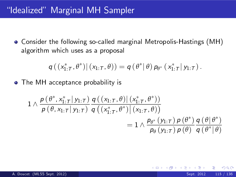
Idealized Marginal MH Sampler
Consider the following so-called marginal Metropolis-Hastings (MH) algorithm which uses as a proposal q ( (x1:T , )j (x1:T , )) = q ( j ) p ( x1:T j y1:T ) . The MH acceptance probability is 1^ p ( , x1:T j y1:T ) q ( (x1:T , )j (x1:T , )) p ( , x1:T j y1:T ) q (x1:T , ) (x1:T , )
= 1^
p (y1:T ) p ( ) q ( j ) p (y1:T ) p ( ) q ( j )
A. Doucet (MLSS Sept. 2012)
Sept. 2012
115 / 136
345
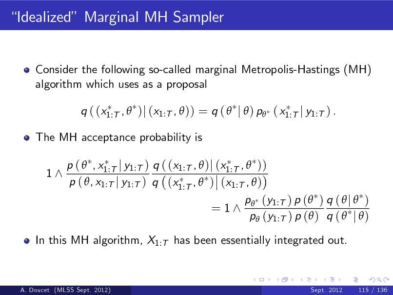
Idealized Marginal MH Sampler
Consider the following so-called marginal Metropolis-Hastings (MH) algorithm which uses as a proposal q ( (x1:T , )j (x1:T , )) = q ( j ) p ( x1:T j y1:T ) . The MH acceptance probability is 1^ p ( , x1:T j y1:T ) q ( (x1:T , )j (x1:T , )) p ( , x1:T j y1:T ) q (x1:T , ) (x1:T , )
= 1^
p (y1:T ) p ( ) q ( j ) p (y1:T ) p ( ) q ( j )
In this MH algorithm, X1:T has been essentially integrated out.
A. Doucet (MLSS Sept. 2012)
Sept. 2012
115 / 136
346
Implementation Issues
Problem 1: We do not know p (y1:T ) = analytically.
R
p (x1:T , y1:T ) dx1:T
A. Doucet (MLSS Sept. 2012)
Sept. 2012
116 / 136
347
Implementation Issues
Problem 1: We do not know p (y1:T ) = analytically.
Problem 2: We do not know how to sample from p ( x1:T j y1:T ) .
R
p (x1:T , y1:T ) dx1:T
A. Doucet (MLSS Sept. 2012)
Sept. 2012
116 / 136
348
Implementation Issues
Problem 1: We do not know p (y1:T ) = analytically.
Problem 2: We do not know how to sample from p ( x1:T j y1:T ) .
R
p (x1:T , y1:T ) dx1:T
Idea: Use SMC approximations of p ( x1:T j y1:T ) and p (y1:T ).
A. Doucet (MLSS Sept. 2012)
Sept. 2012
116 / 136
349

Sequential Monte Carlo aka Particle Filters
Given , SMC methods provide approximations of p ( x1:T j y1:T ) and p (y1:T ).
A. Doucet (MLSS Sept. 2012)
Sept. 2012
117 / 136
350

Sequential Monte Carlo aka Particle Filters
Given , SMC methods provide approximations of p ( x1:T j y1:T ) and p (y1:T ). At time T , we obtain the following approximation of the posterior of interest 1 N p ( x1:T j y1:T ) = b (k ) (x1:T ) N k X 1:T =1 and an approximation of p (y1:T ) is given by p (y1:T ) = p (y1 ) p ( yt j y1:t b b b
t =2 1) T 1)
=
t =1
T
1 N
k =1
N
g
(k ) yt j Xt
!
if we use f ( xt j xt
as a proposal.
A. Doucet (MLSS Sept. 2012)
Sept. 2012
117 / 136
351
![Slide: Reminder...
Under mixing assumptions, we have V [p (y1:T )] b 2 p (y1:T ) D T . N
A. Doucet (MLSS Sept. 2012)
Sept. 2012
118 / 136](https://yosinski.com/mlss12/media/slides/MLSS-2012-Doucet-Sequential-Monte-Carlo-Methods_352.png)
Reminder...
Under mixing assumptions, we have V [p (y1:T )] b 2 p (y1:T ) D T . N
A. Doucet (MLSS Sept. 2012)
Sept. 2012
118 / 136
352
![Slide: Reminder...
Under mixing assumptions, we have V [p (y1:T )] b 2 p (y1:T ) D T . N
Under mixing assumptions, we also have
Z
so if I run an SMC method to obtain p ( x1:T j y1:T ) then b X1:T p ( x1:T j y1:T ), unconditionally X1:T b E [p ( j y1:T )]. b
b jE [p ( x1:T j y1:T )]
p ( x1:T j y1:T )j dx1:T
C
T N
A. Doucet (MLSS Sept. 2012)
Sept. 2012
118 / 136](https://yosinski.com/mlss12/media/slides/MLSS-2012-Doucet-Sequential-Monte-Carlo-Methods_353.png)
Reminder...
Under mixing assumptions, we have V [p (y1:T )] b 2 p (y1:T ) D T . N
Under mixing assumptions, we also have
Z
so if I run an SMC method to obtain p ( x1:T j y1:T ) then b X1:T p ( x1:T j y1:T ), unconditionally X1:T b E [p ( j y1:T )]. b
b jE [p ( x1:T j y1:T )]
p ( x1:T j y1:T )j dx1:T
C
T N
A. Doucet (MLSS Sept. 2012)
Sept. 2012
118 / 136
353
![Slide: Reminder...
Under mixing assumptions, we have V [p (y1:T )] b 2 p (y1:T ) D T . N
Under mixing assumptions, we also have
Z
so if I run an SMC method to obtain p ( x1:T j y1:T ) then b X1:T p ( x1:T j y1:T ), unconditionally X1:T b E [p ( j y1:T )]. b
b jE [p ( x1:T j y1:T )]
p ( x1:T j y1:T )j dx1:T
C
T N
Problem: We cannot compute analytically the particle lter proposal q ( x1:T j y1:T ) = E [p ( x1:T j y1:T )] as it involves an expectation w.r.t b all the variables appearing in the particle algorithm...
Sept. 2012 118 / 136
A. Doucet (MLSS Sept. 2012)](https://yosinski.com/mlss12/media/slides/MLSS-2012-Doucet-Sequential-Monte-Carlo-Methods_354.png)
Reminder...
Under mixing assumptions, we have V [p (y1:T )] b 2 p (y1:T ) D T . N
Under mixing assumptions, we also have
Z
so if I run an SMC method to obtain p ( x1:T j y1:T ) then b X1:T p ( x1:T j y1:T ), unconditionally X1:T b E [p ( j y1:T )]. b
b jE [p ( x1:T j y1:T )]
p ( x1:T j y1:T )j dx1:T
C
T N
Problem: We cannot compute analytically the particle lter proposal q ( x1:T j y1:T ) = E [p ( x1:T j y1:T )] as it involves an expectation w.r.t b all the variables appearing in the particle algorithm...
Sept. 2012 118 / 136
A. Doucet (MLSS Sept. 2012)
354
Idealized Marginal MH Sampler
At iteration i Sample q ( j (i 1)).
A. Doucet (MLSS Sept. 2012)
Sept. 2012
119 / 136
355
Idealized Marginal MH Sampler
At iteration i Sample Sample X1:T q ( j (i 1)). p ( x1:T j y1:T ) .
A. Doucet (MLSS Sept. 2012)
Sept. 2012
119 / 136
356
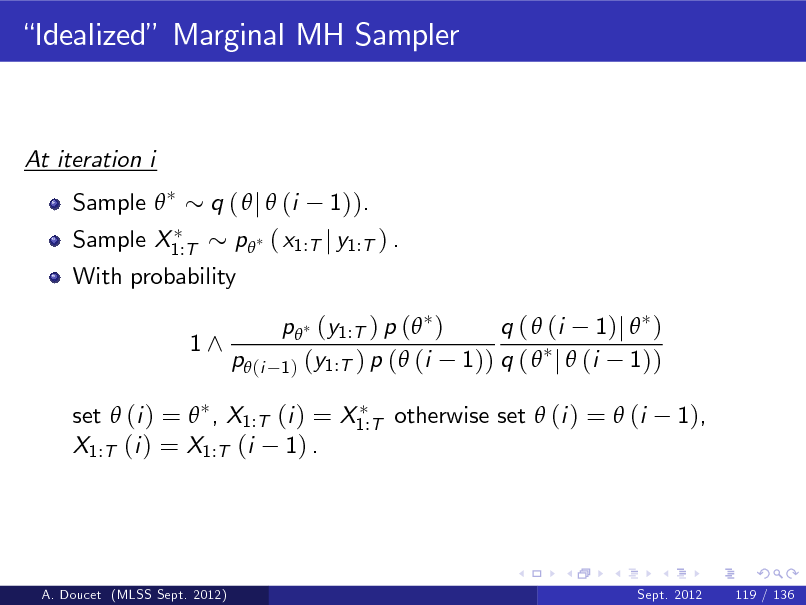
Idealized Marginal MH Sampler
At iteration i Sample Sample X1:T q ( j (i 1)). p ( x1:T j y1:T ) . p (y1:T ) p ( ) q ( (i 1)j ) 1)) q ( j (i 1)) 1 ) (y1:T ) p ( (i 1),
With probability 1^
p (i
set (i ) = , X1:T (i ) = X1:T otherwise set (i ) = (i X1:T (i ) = X1:T (i 1) .
A. Doucet (MLSS Sept. 2012)
Sept. 2012
119 / 136
357
Particle Marginal MH Sampler
At iteration i Sample q ( j (i 1)) and run an SMC algorithm to obtain p ( x1:T j y1:T ) and p (y1:T ). b b
A. Doucet (MLSS Sept. 2012)
Sept. 2012
120 / 136
358
Particle Marginal MH Sampler
At iteration i Sample q ( j (i 1)) and run an SMC algorithm to obtain p ( x1:T j y1:T ) and p (y1:T ). b b Sample X1:T p ( x1:T j y1:T ) . b
A. Doucet (MLSS Sept. 2012)
Sept. 2012
120 / 136
359
Particle Marginal MH Sampler
At iteration i Sample q ( j (i 1)) and run an SMC algorithm to obtain p ( x1:T j y1:T ) and p (y1:T ). b b Sample X1:T With probability 1^ p ( x1:T j y1:T ) . b p (y1:T ) p ( ) b q ( (i 1)j ) 1)) q ( j (i 1)) 1 ) (y1:T ) p ( (i
set (i ) = , X1:T (i ) = X1:T otherwise set (i ) = (i X1:T (i ) = X1:T (i 1) .
p (i b
1),
A. Doucet (MLSS Sept. 2012)
Sept. 2012
120 / 136
360

Validity of the Particle Marginal MH Sampler
Proposition. Assume that the idealizedmarginal MH sampler chain is ergodic then, under very weak assumptions, the PMMH sampler chain is ergodic and admits p ( , x1:T j y1:T ) whatever being N 1.
A. Doucet (MLSS Sept. 2012)
Sept. 2012
121 / 136
361

Validity of the Particle Marginal MH Sampler
Proposition. Assume that the idealizedmarginal MH sampler chain is ergodic then, under very weak assumptions, the PMMH sampler chain is ergodic and admits p ( , x1:T j y1:T ) whatever being N 1. It is easy to show the simpler result that the PMMH admits p ( j y1:T ) as invariant distribution whatever being N 1.
A. Doucet (MLSS Sept. 2012)
Sept. 2012
121 / 136
362

Validity of the Particle Marginal MH Sampler
Proposition. Assume that the idealizedmarginal MH sampler chain is ergodic then, under very weak assumptions, the PMMH sampler chain is ergodic and admits p ( , x1:T j y1:T ) whatever being N 1. It is easy to show the simpler result that the PMMH admits p ( j y1:T ) as invariant distribution whatever being N 1.
Z
Let U denote all the r.v. introduce to build the SMC estimate then write p (y1:T ) = p (y1:T , U ) and from unbiasedness b b p (y1:T , u ) q (u ) du = p (y1:T ) . b
A. Doucet (MLSS Sept. 2012)
Sept. 2012
121 / 136
363

An Incomplete But Trivial Proof
The PMMH targets the distribution e (, u ) p ( ) p (y1:T , u ) q (u ) b e ( ) = p ( j y1:T ).
which satises
A. Doucet (MLSS Sept. 2012)
Sept. 2012
122 / 136
364
An Incomplete But Trivial Proof
The PMMH targets the distribution e (, u ) p ( ) p (y1:T , u ) q (u ) b e ( ) = p ( j y1:T ).
which satises
The PMMH sampler uses as a proposal
q ( ( , u )j (, u )) = q ( j ) q (u ) and
e ( ,u ) q ( (,u )j( ,u )) e (,u ) q ( ( ,u )j(,u ))
=
p ( )p (y1:T ,u )q (u ) q ( j )q (u ) b p ( )p (y1:T ,u )q (u ) q ( j )q (u ) b b q 1:T ,u = p (())pp ((yy1:T ,u ) ) q ( j ) p b ( j )
A. Doucet (MLSS Sept. 2012)
Sept. 2012
122 / 136
365
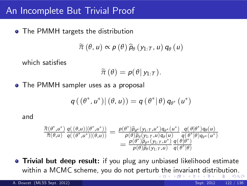
An Incomplete But Trivial Proof
The PMMH targets the distribution e (, u ) p ( ) p (y1:T , u ) q (u ) b e ( ) = p ( j y1:T ).
which satises
The PMMH sampler uses as a proposal
q ( ( , u )j (, u )) = q ( j ) q (u ) and
e ( ,u ) q ( (,u )j( ,u )) e (,u ) q ( ( ,u )j(,u ))
=
Trivial but deep result: if you plug any unbiased likelihood estimate within a MCMC scheme, you do not perturb the invariant distribution.
A. Doucet (MLSS Sept. 2012) Sept. 2012 122 / 136
p ( )p (y1:T ,u )q (u ) q ( j )q (u ) b p ( )p (y1:T ,u )q (u ) q ( j )q (u ) b b q 1:T ,u = p (())pp ((yy1:T ,u ) ) q ( j ) p b ( j )
366

Explicit Structure of the Target Distribution
Let rst consider the case where T = 1.
A. Doucet (MLSS Sept. 2012)
Sept. 2012
123 / 136
367
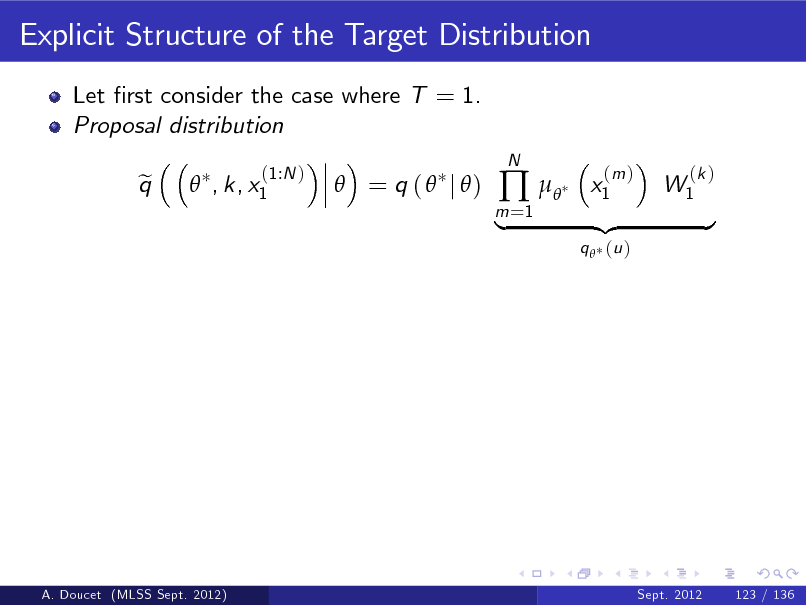
Explicit Structure of the Target Distribution
Let rst consider the case where T = 1. Proposal distribution q e , k, x1
(1:N )
= q ( j )
m =1
N
x1
(m )
W1
(k )
|
q (u )
{z
}
A. Doucet (MLSS Sept. 2012)
Sept. 2012
123 / 136
368
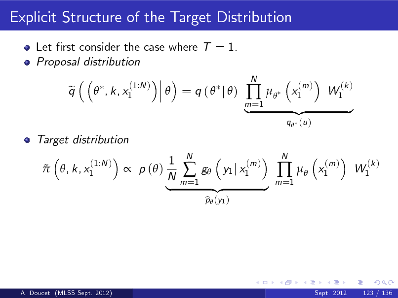
Explicit Structure of the Target Distribution
Let rst consider the case where T = 1. Proposal distribution q e , k, x1
(1:N )
= q ( j )
m =1
N
x1
(m )
W1
(k )
Target distribution , k, x1
(1:N )
|
q (u )
{z
} x1
(m )
p ( )
1 N |
m =1
N
g y1 j x1
p (y 1 ) b
(m )
{z
}
m =1
N
W1
(k )
A. Doucet (MLSS Sept. 2012)
Sept. 2012
123 / 136
369
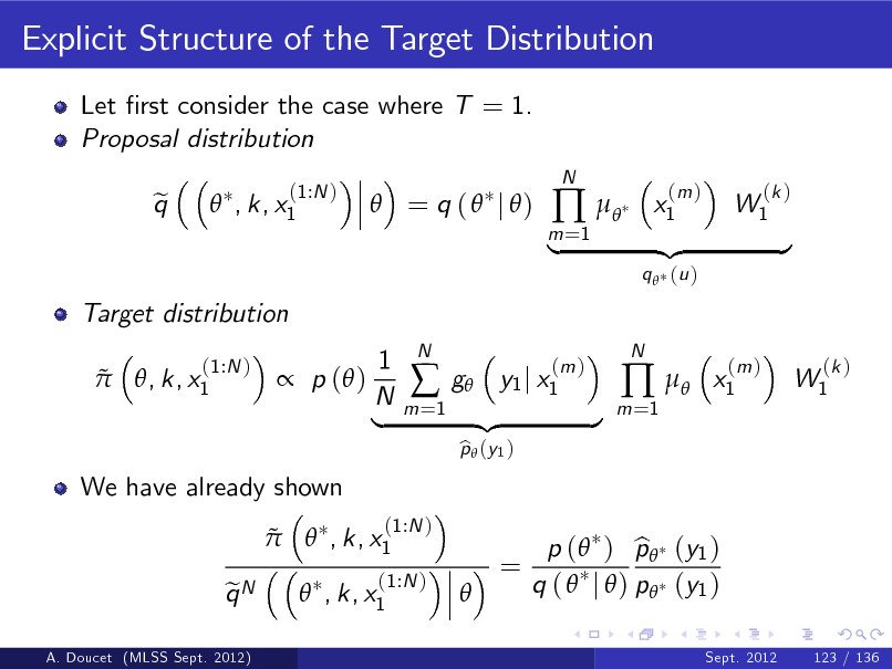
Explicit Structure of the Target Distribution
Let rst consider the case where T = 1. Proposal distribution q e , k, x1
(1:N )
= q ( j )
m =1
N
x1
(m )
W1
(k )
Target distribution , k, x1
(1:N )
|
q (u )
{z
} x1
(m )
p ( )
We have already shown
1 N |
m =1
N
g y1 j x1
p (y 1 ) b
(m )
{z
}
m =1
N
W1
(k )
, k, x1 qN e
(1:N )
(1:N ) , k, x1
=
p ( ) p (y1 ) b q ( j ) p (y1 )
Sept. 2012 123 / 136
A. Doucet (MLSS Sept. 2012)
370
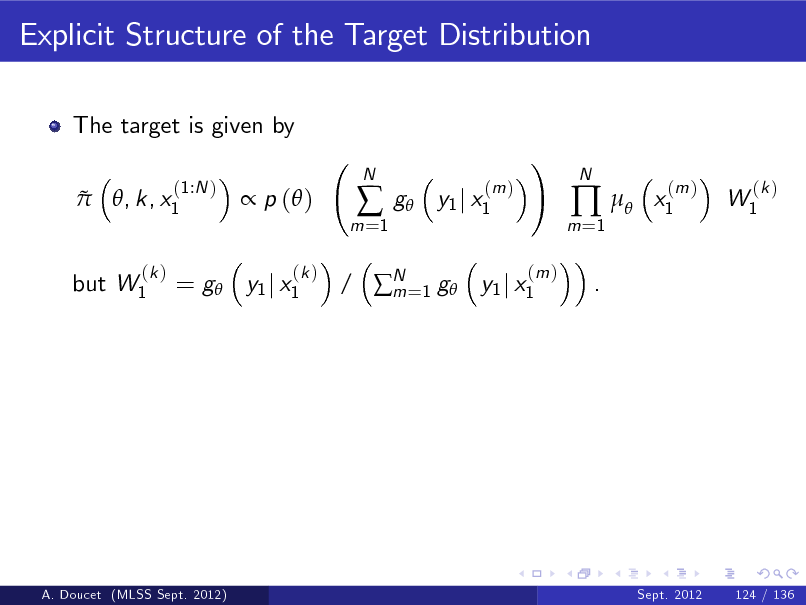
Explicit Structure of the Target Distribution
The target is given by
(1:N ) , k, x1
p ( )
(k )
m =1
N
g
(m ) y1 j x1
!
(m )
m =1
.
N
x1
(m )
W1
(k )
but W1
(k )
= g y1 j x1
/ N =1 g y1 j x1 m
A. Doucet (MLSS Sept. 2012)
Sept. 2012
124 / 136
371
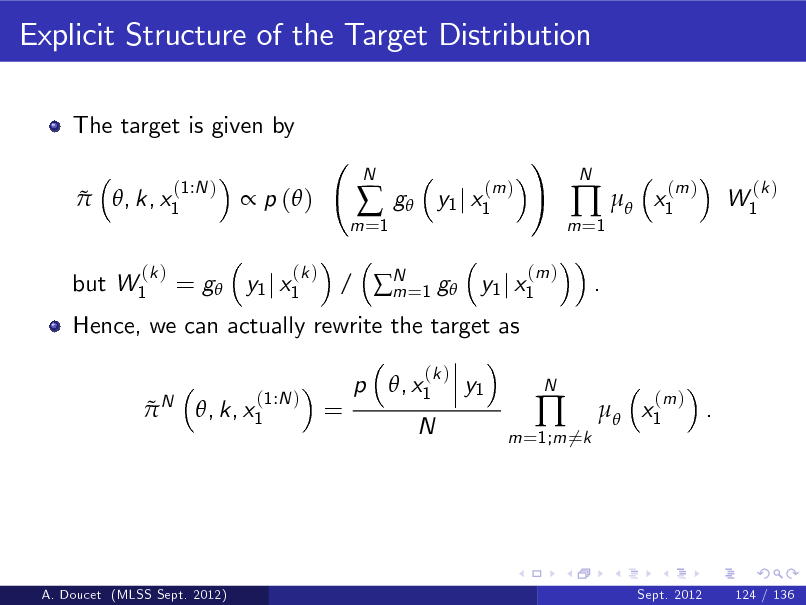
Explicit Structure of the Target Distribution
The target is given by
(1:N ) , k, x1
p ( )
(k )
m =1
N
g
(m ) y1 j x1
!
(m )
m =1
.
N
x1
(m )
W1
(k )
but W1
(k )
Hence, we can actually rewrite the target as
N
= g y1 j x1
/ N =1 g y1 j x1 m p , x1
(k )
(1:N ) , k, x1
=
y1
N
m =1;m 6=k
N
x1
(m )
.
A. Doucet (MLSS Sept. 2012)
Sept. 2012
124 / 136
372
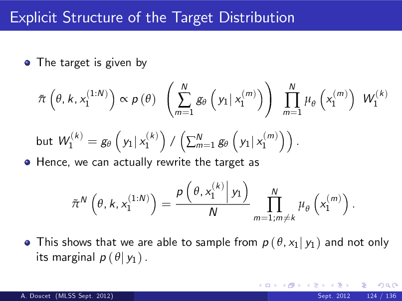
Explicit Structure of the Target Distribution
The target is given by
(1:N ) , k, x1
p ( )
(k )
m =1
N
g
(m ) y1 j x1
!
(m )
m =1
.
N
x1
(m )
W1
(k )
but W1
(k )
Hence, we can actually rewrite the target as
N
= g y1 j x1
/ N =1 g y1 j x1 m p , x1
(k )
(1:N ) , k, x1
=
y1
N
m =1;m 6=k
N
x1
(m )
.
This shows that we are able to sample from p ( , x1 j y1 ) and not only its marginal p ( j y1 ) .
A. Doucet (MLSS Sept. 2012) Sept. 2012 124 / 136
373

Sampling from the Target Distribution
To sample from this target distribution
A. Doucet (MLSS Sept. 2012)
Sept. 2012
125 / 136
374

Sampling from the Target Distribution
To sample from this target distribution
Sample K from a uniform distribution on f1, ..., N g.
A. Doucet (MLSS Sept. 2012)
Sept. 2012
125 / 136
375

Sampling from the Target Distribution
To sample from this target distribution
Sample , X1 from p ( , x1 j y1 ). (We do not know how to do this, this is why we use MCMC). Sample K from a uniform distribution on f1, ..., N g.
(K )
A. Doucet (MLSS Sept. 2012)
Sept. 2012
125 / 136
376

Sampling from the Target Distribution
To sample from this target distribution
Sample , X1 from p ( , x1 j y1 ). (We do not know how to do this, this is why we use MCMC). Sample K from a uniform distribution on f1, ..., N g.
(K )
Sample X1
(m )
(x1 ) for m 6= K .
A. Doucet (MLSS Sept. 2012)
Sept. 2012
125 / 136
377

Explicit Structure of the Target Distribution
This construction can be extended to the case T > 1.
A. Doucet (MLSS Sept. 2012)
Sept. 2012
126 / 136
378

Explicit Structure of the Target Distribution
This construction can be extended to the case T > 1. To sample from this target distribution
A. Doucet (MLSS Sept. 2012)
Sept. 2012
126 / 136
379

Explicit Structure of the Target Distribution
This construction can be extended to the case T > 1. To sample from this target distribution
Sample indexes from a uniform distribution on f1, ..., N gT corresponding to an ancestral line.
A. Doucet (MLSS Sept. 2012)
Sept. 2012
126 / 136
380

Explicit Structure of the Target Distribution
This construction can be extended to the case T > 1. To sample from this target distribution
Sample indexes from a uniform distribution on f1, ..., N gT corresponding to an ancestral line. Sample and X1 :T for this ancestral line from p ( , x1 :T j y1 :T ). (We do not know how to do this, this is why we use MCMC).
A. Doucet (MLSS Sept. 2012)
Sept. 2012
126 / 136
381

Explicit Structure of the Target Distribution
This construction can be extended to the case T > 1. To sample from this target distribution
Sample indexes from a uniform distribution on f1, ..., N gT corresponding to an ancestral line. Sample and X1 :T for this ancestral line from p ( , x1 :T j y1 :T ). (We do not know how to do this, this is why we use MCMC).
Run a conditional SMC algorithm compatible with X1:T and its ancestral lineage; see (Andrieu, D. & Holenstein, 2010).
A. Doucet (MLSS Sept. 2012)
Sept. 2012
126 / 136
382
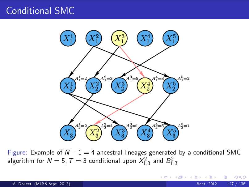
Conditional SMC
Figure: Example of N 1 = 4 ancestral lineages generated by a conditional SMC 2 2 algorithm for N = 5, T = 3 conditional upon X1 :3 and B1 :3
A. Doucet (MLSS Sept. 2012) Sept. 2012 127 / 136
383

Idealized Gibbs Sampler
To sample from p ( , x1:T j y1:T ), an MCMC strategy consists of using the following block Gibbs sampler. At iteration i
A. Doucet (MLSS Sept. 2012)
Sept. 2012
128 / 136
384

Idealized Gibbs Sampler
To sample from p ( , x1:T j y1:T ), an MCMC strategy consists of using the following block Gibbs sampler. At iteration i Sample X1:T (i ) p (i
1)
( x1:T j y1:T ).
A. Doucet (MLSS Sept. 2012)
Sept. 2012
128 / 136
385

Idealized Gibbs Sampler
To sample from p ( , x1:T j y1:T ), an MCMC strategy consists of using the following block Gibbs sampler. At iteration i Sample X1:T (i ) Sample (i )
( x1:T j y1:T ). p ( j y1:T , X1:T (i )) .
p (i
1)
A. Doucet (MLSS Sept. 2012)
Sept. 2012
128 / 136
386
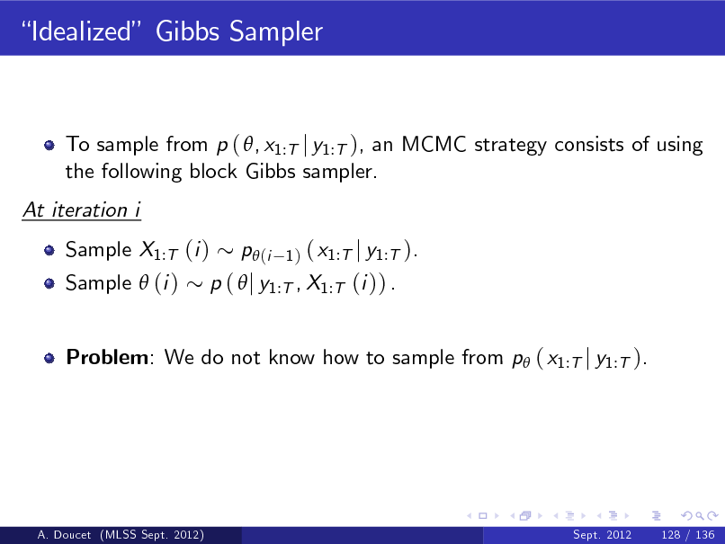
Idealized Gibbs Sampler
To sample from p ( , x1:T j y1:T ), an MCMC strategy consists of using the following block Gibbs sampler. At iteration i Sample X1:T (i ) Sample (i )
( x1:T j y1:T ). p ( j y1:T , X1:T (i )) .
p (i
1)
Problem: We do not know how to sample from p ( x1:T j y1:T ).
A. Doucet (MLSS Sept. 2012)
Sept. 2012
128 / 136
387
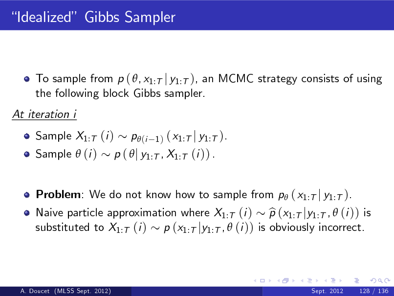
Idealized Gibbs Sampler
To sample from p ( , x1:T j y1:T ), an MCMC strategy consists of using the following block Gibbs sampler. At iteration i Sample X1:T (i ) Sample (i )
( x1:T j y1:T ). p ( j y1:T , X1:T (i )) .
p (i
1)
Problem: We do not know how to sample from p ( x1:T j y1:T ).
Naive particle approximation where X1:T (i ) p (x1:T jy1:T , (i )) is b substituted to X1:T (i ) p (x1:T jy1:T , (i )) is obviously incorrect.
A. Doucet (MLSS Sept. 2012)
Sept. 2012
128 / 136
388
Particle Gibbs Sampler
At iteration i Sample (i ) p ( jy1:T , X1:T (i 1)).
A. Doucet (MLSS Sept. 2012)
Sept. 2012
129 / 136
389
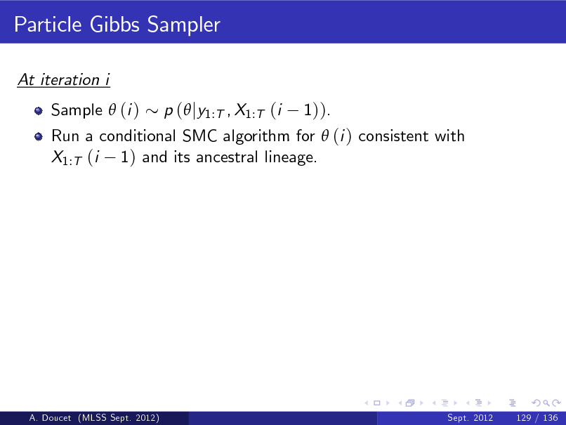
Particle Gibbs Sampler
At iteration i Sample (i ) Run a conditional SMC algorithm for (i ) consistent with X1:T (i 1) and its ancestral lineage. p ( jy1:T , X1:T (i 1)).
A. Doucet (MLSS Sept. 2012)
Sept. 2012
129 / 136
390
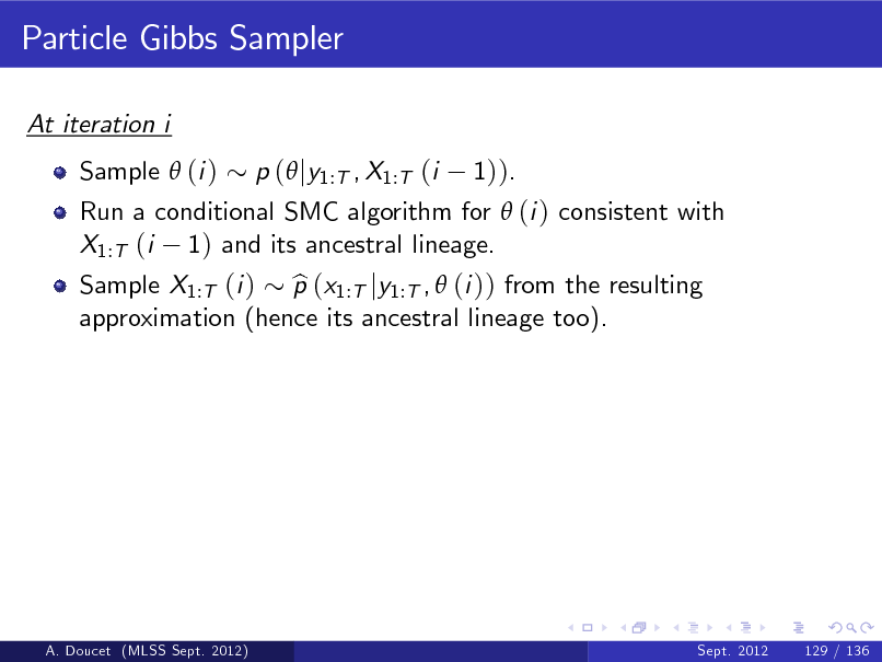
Particle Gibbs Sampler
At iteration i Sample (i ) Run a conditional SMC algorithm for (i ) consistent with X1:T (i 1) and its ancestral lineage. Sample X1:T (i ) p (x1:T jy1:T , (i )) from the resulting b approximation (hence its ancestral lineage too). p ( jy1:T , X1:T (i 1)).
A. Doucet (MLSS Sept. 2012)
Sept. 2012
129 / 136
391
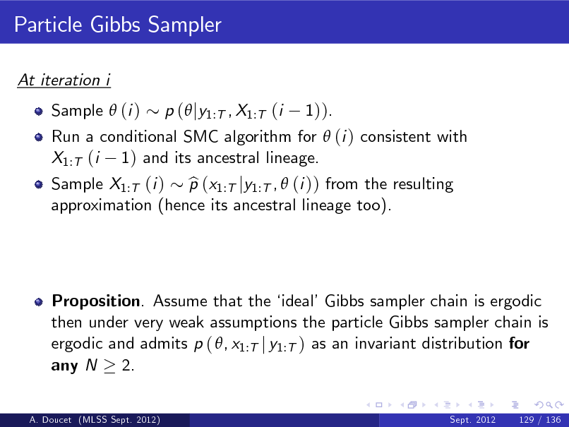
Particle Gibbs Sampler
At iteration i Sample (i ) Run a conditional SMC algorithm for (i ) consistent with X1:T (i 1) and its ancestral lineage. Sample X1:T (i ) p (x1:T jy1:T , (i )) from the resulting b approximation (hence its ancestral lineage too). p ( jy1:T , X1:T (i 1)).
Proposition. Assume that the idealGibbs sampler chain is ergodic then under very weak assumptions the particle Gibbs sampler chain is ergodic and admits p ( , x1:T j y1:T ) as an invariant distribution for any N 2.
A. Doucet (MLSS Sept. 2012) Sept. 2012 129 / 136
392

Nonlinear State-Space Model
Consider the following model Xt Yt where Vt
= =
1 Xt 2
1
+ 25
Xt 1 1 + Xt2
+ 8 cos 1.2t + Vt ,
1
Xt2 + Wt 20
N 0, 2 , Wt v
N 0, 2 and X1 w
N 0, 52 .
A. Doucet (MLSS Sept. 2012)
Sept. 2012
130 / 136
393

Nonlinear State-Space Model
Consider the following model Xt Yt where Vt
= =
1 Xt 2
1
+ 25
Xt 1 1 + Xt2
+ 8 cos 1.2t + Vt ,
1
Xt2 + Wt 20
N 0, 2 , Wt N 0, 2 and X1 v w Use the prior for fXt g as proposal distribution.
N 0, 52 .
A. Doucet (MLSS Sept. 2012)
Sept. 2012
130 / 136
394

Nonlinear State-Space Model
Consider the following model Xt Yt where Vt
= =
1 Xt 2
1
+ 25
Xt 1 1 + Xt2
+ 8 cos 1.2t + Vt ,
1
Xt2 + Wt 20
N 0, 2 , Wt N 0, 2 and X1 N 0, 52 . v w Use the prior for fXt g as proposal distribution. For a xed , we evaluate the expected acceptance probability as a function of N.
A. Doucet (MLSS Sept. 2012)
Sept. 2012
130 / 136
395
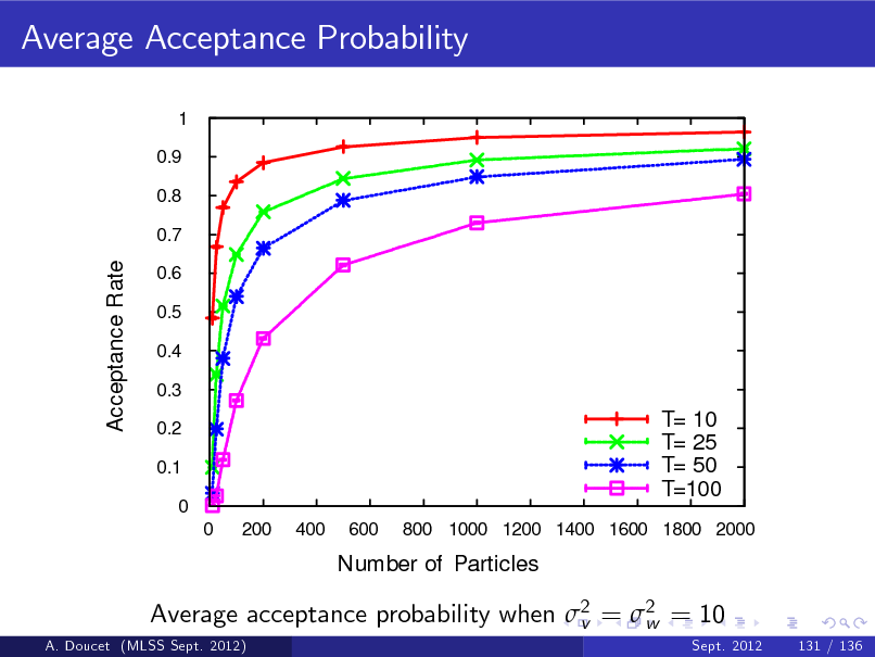
Average Acceptance Probability
1 0.9 0.8 0.7
Acceptance Rate
0.6 0.5 0.4 0.3 0.2 0.1 0 0 200 400 600
T= 10 T= 25 T= 50 T=100
800 1000 1200 1400 1600 1800 2000
Number of Particles
Average acceptance probability when 2 = 2 = 10 v w
A. Doucet (MLSS Sept. 2012) Sept. 2012 131 / 136
396
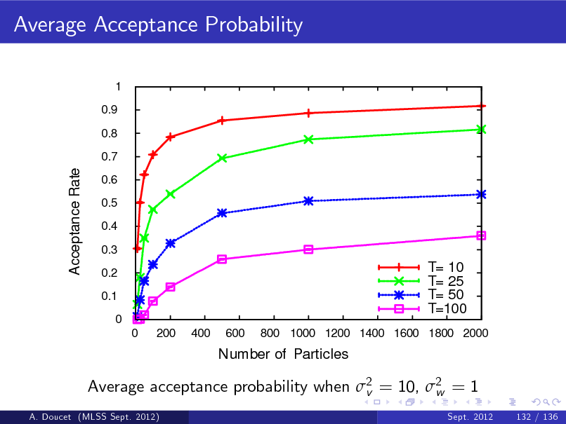
Average Acceptance Probability
1 0.9 0.8 0.7
Acceptance Rate
0.6 0.5 0.4 0.3 0.2 0.1 0 0 200 400 600
T= 10 T= 25 T= 50 T=100
800 1000 1200 1400 1600 1800 2000
Number of Particles
Average acceptance probability when 2 = 10, 2 = 1 v w
A. Doucet (MLSS Sept. 2012) Sept. 2012 132 / 136
397
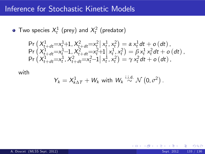
Inference for Stochastic Kinetic Models
Two species Xt1 (prey) and Xt2 (predator) Pr Xt1+dt =xt1+1, Xt2+dt =xt2 xt1 , xt2 = xt1 dt + o (dt ) , Pr Xt1+dt =xt1 1, Xt2+dt =xt2+1 xt1 , xt2 = xt1 xt2 dt + o (dt ) , Pr Xt1+dt =xt1 , Xt2+dt =xt2 1 xt1 , xt2 = xt2 dt + o (dt ) , with
1 Yk = Xk T + Wk with Wk i.i.d.
N 0, 2 .
A. Doucet (MLSS Sept. 2012)
Sept. 2012
133 / 136
398
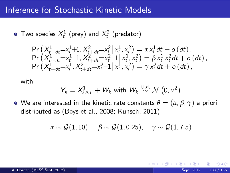
Inference for Stochastic Kinetic Models
Two species Xt1 (prey) and Xt2 (predator) Pr Xt1+dt =xt1+1, Xt2+dt =xt2 xt1 , xt2 = xt1 dt + o (dt ) , Pr Xt1+dt =xt1 1, Xt2+dt =xt2+1 xt1 , xt2 = xt1 xt2 dt + o (dt ) , Pr Xt1+dt =xt1 , Xt2+dt =xt2 1 xt1 , xt2 = xt2 dt + o (dt ) , with
1 Yk = Xk T + Wk with Wk i.i.d.
N 0, 2 .
We are interested in the kinetic rate constants = (, , ) a priori distributed as (Boys et al., 2008; Kunsch, 2011)
G(1, 10),
G(1, 0.25),
G(1, 7.5).
A. Doucet (MLSS Sept. 2012)
Sept. 2012
133 / 136
399
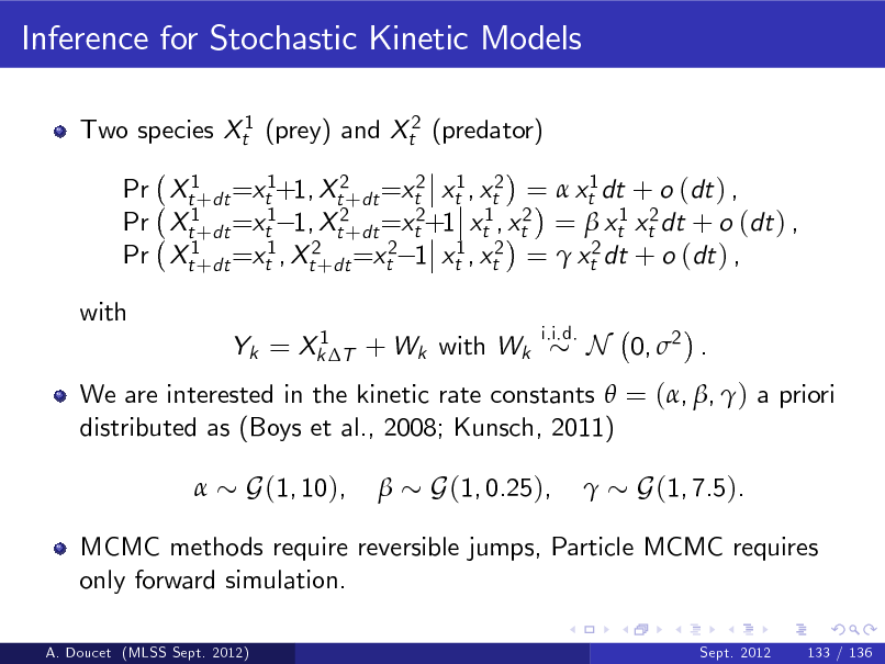
Inference for Stochastic Kinetic Models
Two species Xt1 (prey) and Xt2 (predator) Pr Xt1+dt =xt1+1, Xt2+dt =xt2 xt1 , xt2 = xt1 dt + o (dt ) , Pr Xt1+dt =xt1 1, Xt2+dt =xt2+1 xt1 , xt2 = xt1 xt2 dt + o (dt ) , Pr Xt1+dt =xt1 , Xt2+dt =xt2 1 xt1 , xt2 = xt2 dt + o (dt ) , with
1 Yk = Xk T + Wk with Wk i.i.d.
N 0, 2 .
We are interested in the kinetic rate constants = (, , ) a priori distributed as (Boys et al., 2008; Kunsch, 2011)
G(1, 10),
G(1, 0.25),
G(1, 7.5).
MCMC methods require reversible jumps, Particle MCMC requires only forward simulation.
A. Doucet (MLSS Sept. 2012) Sept. 2012 133 / 136
400
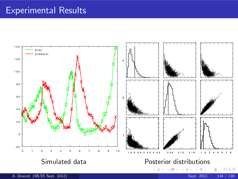
Experimental Results
140 prey predat or 120
100
80
60
40
20
0
-20 0 1 2 3 4 5 6 7 8 9 10
1 .5 2 2 .5 3 3 .5 4 4 .5 0 .0 6 0 .1 2 0 .1 8 1 2 3 4 5 6 7 8
Simulated data
A. Doucet (MLSS Sept. 2012)
Posterior distributions
Sept. 2012 134 / 136
401
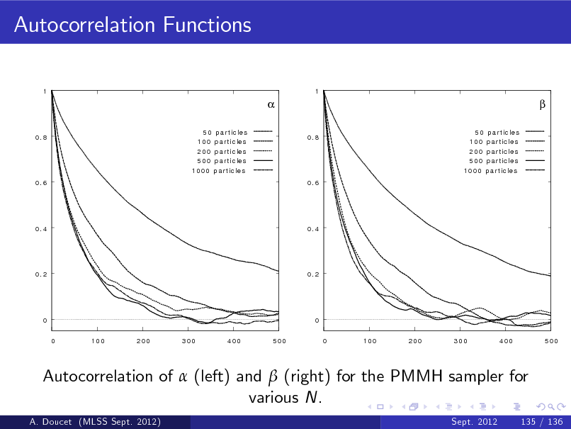
Autocorrelation Functions
1 1
0.8 50 100 200 500 1000 p a r t ic le s p a r t ic le s p a r t ic le s p a r t ic le s p a r t ic le s 0.8 50 100 200 500 1000 p a r t ic le s p a r t ic le s p a r t ic le s p a r t ic le s p a r t ic le s
0.6
0.6
0.4
0.4
0.2
0.2
0 0 100 200 300 400 500
0 0 100 200 300 400 500
Autocorrelation of (left) and (right) for the PMMH sampler for various N.
A. Doucet (MLSS Sept. 2012) Sept. 2012 135 / 136
402

Summary
O- ine Bayesian parameter inference is feasible by using SMC proposals within MCMC.
A. Doucet (MLSS Sept. 2012)
Sept. 2012
136 / 136
403

Summary
O- ine Bayesian parameter inference is feasible by using SMC proposals within MCMC. This approach does not suer from degeneracy problem and N scales roughly linearly with T .
A. Doucet (MLSS Sept. 2012)
Sept. 2012
136 / 136
404
Summary
O- ine Bayesian parameter inference is feasible by using SMC proposals within MCMC. This approach does not suer from degeneracy problem and N scales roughly linearly with T . Particle MCMC allow us to perform Bayesian inference for dynamic models for which only forward simulation is possible.
A. Doucet (MLSS Sept. 2012)
Sept. 2012
136 / 136
405

Summary
O- ine Bayesian parameter inference is feasible by using SMC proposals within MCMC. This approach does not suer from degeneracy problem and N scales roughly linearly with T . Particle MCMC allow us to perform Bayesian inference for dynamic models for which only forward simulation is possible. Computationally intensive but several implementations on GPU already available and applications in control, ecology, econometrics, biochemical systems, epidemiology, water resources research etc.
A. Doucet (MLSS Sept. 2012)
Sept. 2012
136 / 136
406

Summary
O- ine Bayesian parameter inference is feasible by using SMC proposals within MCMC. This approach does not suer from degeneracy problem and N scales roughly linearly with T . Particle MCMC allow us to perform Bayesian inference for dynamic models for which only forward simulation is possible. Computationally intensive but several implementations on GPU already available and applications in control, ecology, econometrics, biochemical systems, epidemiology, water resources research etc. Selection of N is a key issue and some guidelines are available (Lee, Andrieu & D., 2012), (D., Pitt & Kohn, 2012).
A. Doucet (MLSS Sept. 2012)
Sept. 2012
136 / 136
407