An introduction to holonomic gradient method in statistics Akimichi Takemura, Univ. Tokyo September 5, 2012

Items
1. First example: Airy-like function 2. Holonomic function and holonomic gradient method (HGM) 3. Another example: incomplete gamma function 4. Wishart distribution and hypergeometric function of a matrix argument 5. HGM for two-dimensional Wishart matrix 6. Pfaan system for general dimension 7. Numerical experiments
1

Coauthors on HGM: H.Hashiguchi, T.Koyama, H.Nakayama, K.Nishiyama, M.Noro, Y.Numata, K.Ohara, T.Sei, N.Takayama. HGM proposed in Holonomic gradient descent and its application to the Fisher-Bingham integral, Advances in Applied Mathematics, 47, 639658. N3 OST2 . 2011. We have now about 7 manuscripts on HGM, mainly by Takayama group. Wishart discussed in arXiv:1201.0472v3
2

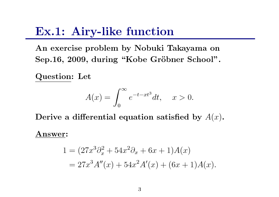
Ex.1: Airy-like function
An exercise problem by Nobuki Takayama on Sep.16, 2009, during Kobe Grbner School. o Question: Let A(x) =
0

e

txt3

dt,

x > 0.

Derive a dierential equation satised by A(x). Answer:
2 1 = (27x3 x + 54x2 x + 6x + 1)A(x)

= 27x3 A (x) + 54x2 A (x) + (6x + 1)A(x).
3

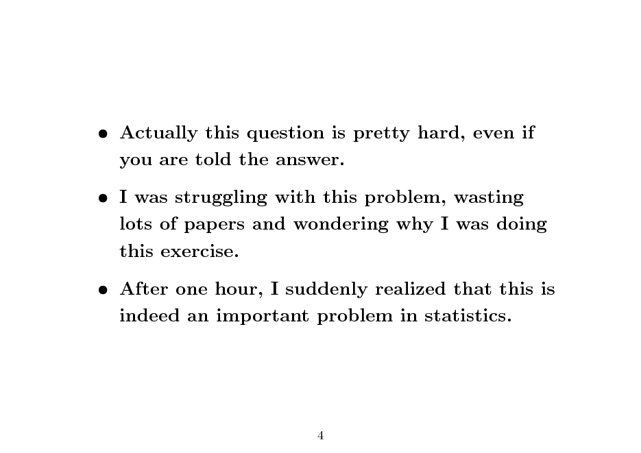
Actually this question is pretty hard, even if you are told the answer. I was struggling with this problem, wasting lots of papers and wondering why I was doing this exercise. After one hour, I suddenly realized that this is indeed an important problem in statistics.

4

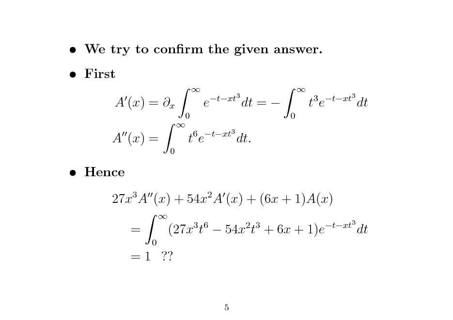
We try to conrm the given answer. First A (x) = x A (x) =
0 0

e

txt3

dt =

0

te

3 txt3

dt

te

6 txt3

dt.

Hence 27x3 A (x) + 54x2 A (x) + (6x + 1)A(x) =
0 3 6 2 3 txt3

(27x t 54x t + 6x + 1)e

dt

= 1 ??

5

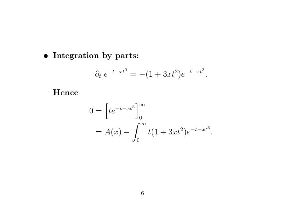
Integration by parts: t e Hence 0 = te
txt3 0 0 txt3

= (1 + 3xt )e

2

txt3

.

= A(x)

t(1 + 3xt )e

2

txt3

.

6

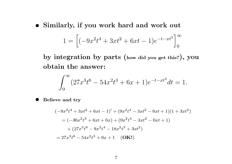
Similarly, if you work hard and work out 1 = (9x t + 3xt + 6xt 1)e
2 4 2 txt3 0

by integration by parts (how did you get this?), you obtain the answer:
0

(27x t 54x t + 6x + 1)e

3 6

2 3

txt3

dt = 1.

Believe and try (9x2 t4 + 3xt2 + 6xt 1) + (9x2 t4 3xt2 6xt + 1)(1 + 3xt2 ) = (36x2 t3 + 6xt + 6x) + (9x2 t4 3xt2 6xt + 1) + (27x3 t6 9x2 t4 18x2 t3 + 3xt2 ) (OK!)

= 27x3 t6 54x2 t3 + 6x + 1

7

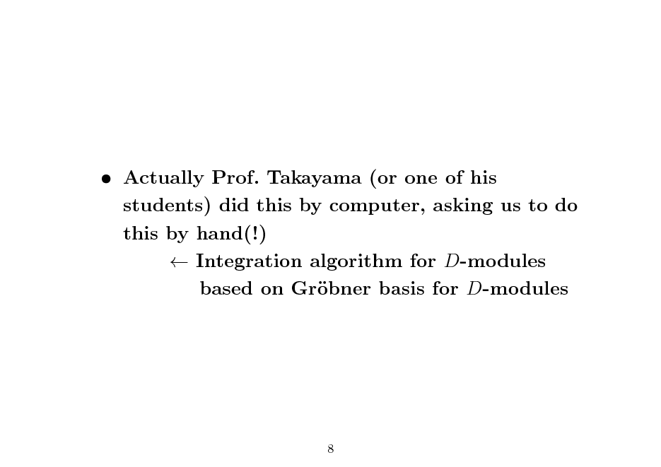
Actually Prof. Takayama (or one of his students) did this by computer, asking us to do this by hand(!) Integration algorithm for D-modules based on Grbner basis for D-modules o

8

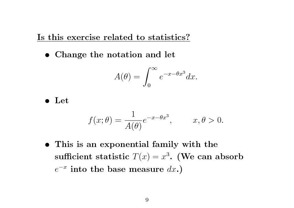
Is this exercise related to statistics? Change the notation and let A() =
0

e

xx3

dx.

Let

1 xx3 f (x; ) = e , A()

x, > 0.

This is an exponential family with the sucient statistic T (x) = x3 . (We can absorb ex into the base measure dx.)

9

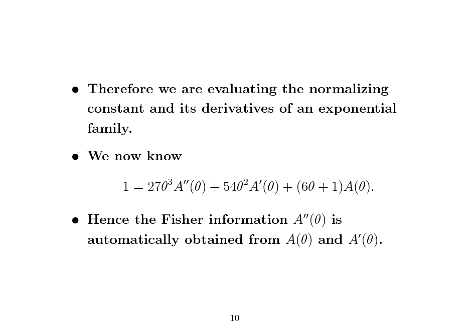
Therefore we are evaluating the normalizing constant and its derivatives of an exponential family. We now know 1 = 273 A () + 542 A () + (6 + 1)A(). Hence the Fisher information A () is automatically obtained from A() and A ().

10

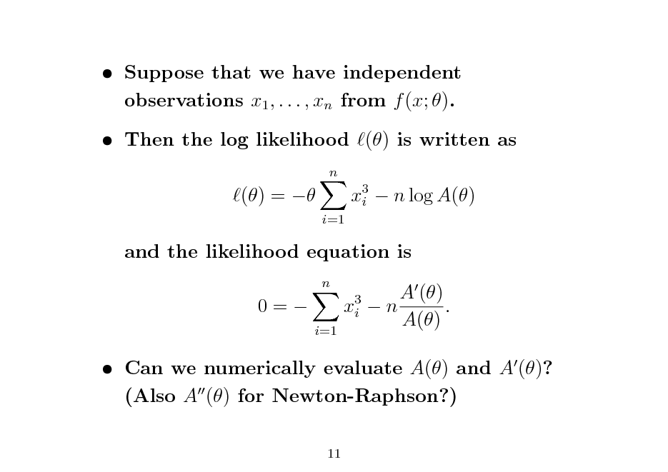
Suppose that we have independent observations x1 , . . . , xn from f (x; ). Then the log likelihood () is written as
n

() =

i=1

x3 n log A() i

and the likelihood equation is
n

0=

x3 i
i=1

A () n . A()

Can we numerically evaluate A() and A ()? (Also A () for Newton-Raphson?)
11

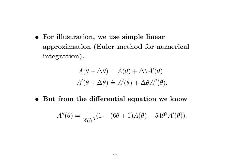
For illustration, we use simple linear approximation (Euler method for numerical integration). . A( + ) = A() + A () . A ( + ) = A () + A (). But from the dierential equation we know 1 A () = (1 (6 + 1)A() 542 A ()). 273

12

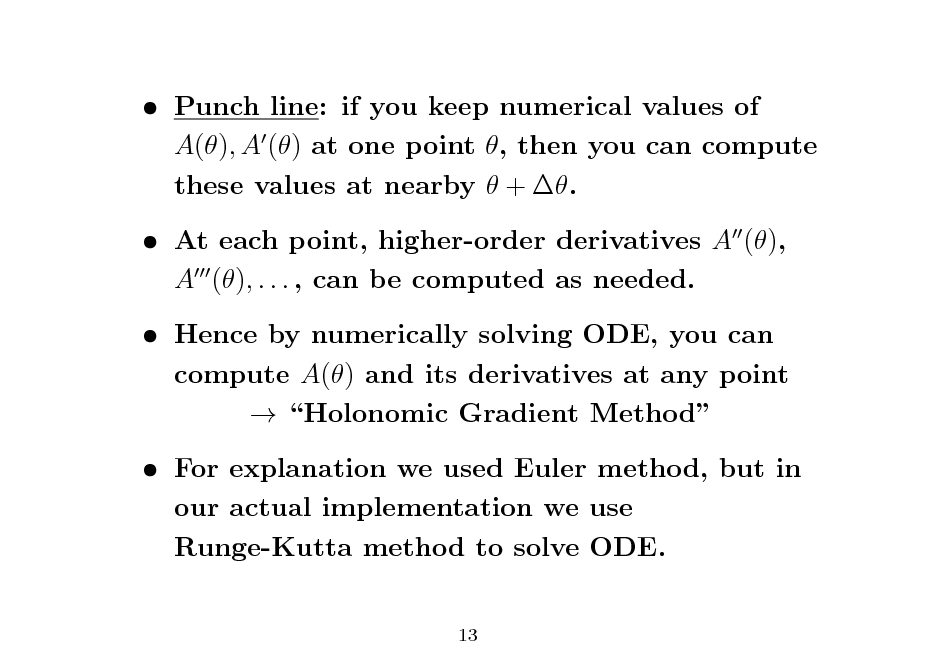
Punch line: if you keep numerical values of A(), A () at one point , then you can compute these values at nearby + . At each point, higher-order derivatives A (), A (), . . . , can be computed as needed. Hence by numerically solving ODE, you can compute A() and its derivatives at any point Holonomic Gradient Method For explanation we used Euler method, but in our actual implementation we use Runge-Kutta method to solve ODE.
13

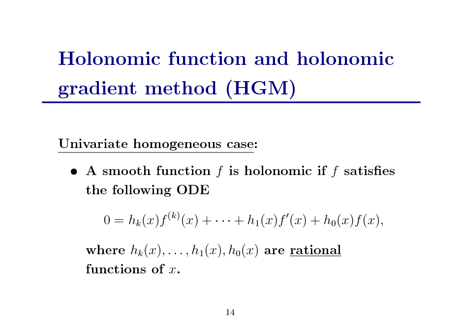
Holonomic function and holonomic gradient method (HGM)
Univariate homogeneous case: A smooth function f is holonomic if f satises the following ODE 0 = hk (x)f (k) (x) + + h1 (x)f (x) + h0 (x)f (x), where hk (x), . . . , h1 (x), h0 (x) are rational functions of x.
14

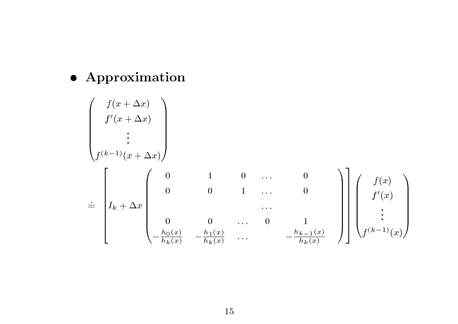
Approximation
f (k1) (x + x) 0 0 . = Ik + x 0 f (x + x) . . .
k

f (x + x)

1 0 0 h1 (x)
k

0 1 ... ...

... ... ... 0

0 0 1
hk1 (x) hk (x)

h0 (x)

h (x)

h (x)

f (x) . . . f (k1) (x)

f (x)

15

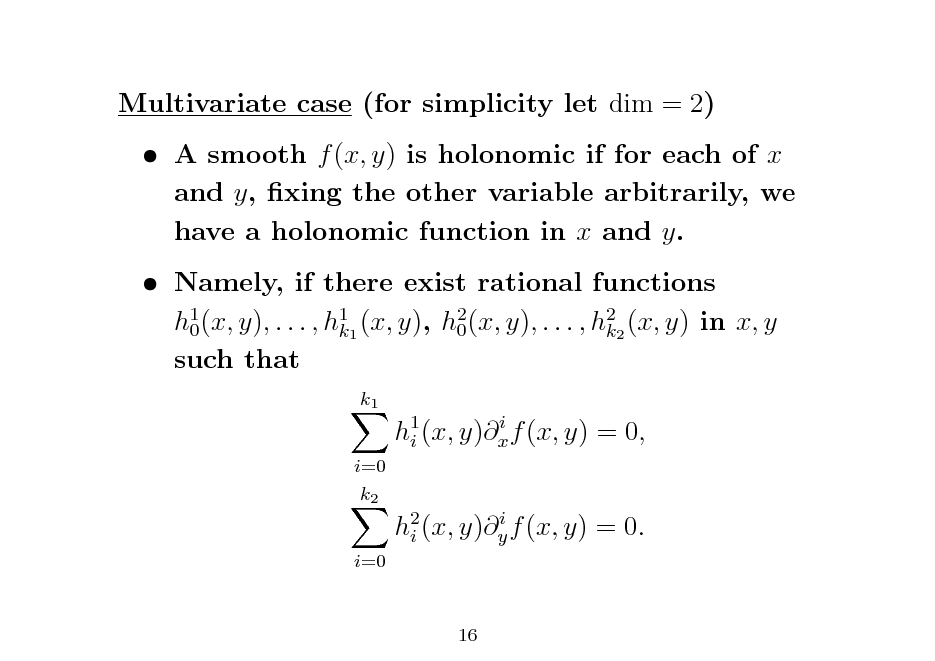
Multivariate case (for simplicity let dim = 2) A smooth f (x, y) is holonomic if for each of x and y, xing the other variable arbitrarily, we have a holonomic function in x and y. Namely, if there exist rational functions h1 (x, y), . . . , h11 (x, y), h2 (x, y), . . . , h22 (x, y) in x, y 0 0 k k such that
k1 i h1 (x, y)x f (x, y) = 0, i i=0 k2 i h2 (x, y)y f (x, y) = 0. i i=0

16

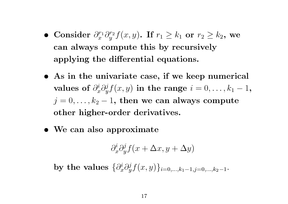
r r Consider x1 y2 f (x, y). If r1 k1 or r2 k2 , we can always compute this by recursively applying the dierential equations.

As in the univariate case, if we keep numerical i j values of x y f (x, y) in the range i = 0, . . . , k1 1, j = 0, . . . , k2 1, then we can always compute other higher-order derivatives. We can also approximate
i j x y f (x + x, y + y) i j by the values {x y f (x, y)}i=0,...,k1 1,j=0,...,k2 1 .

17

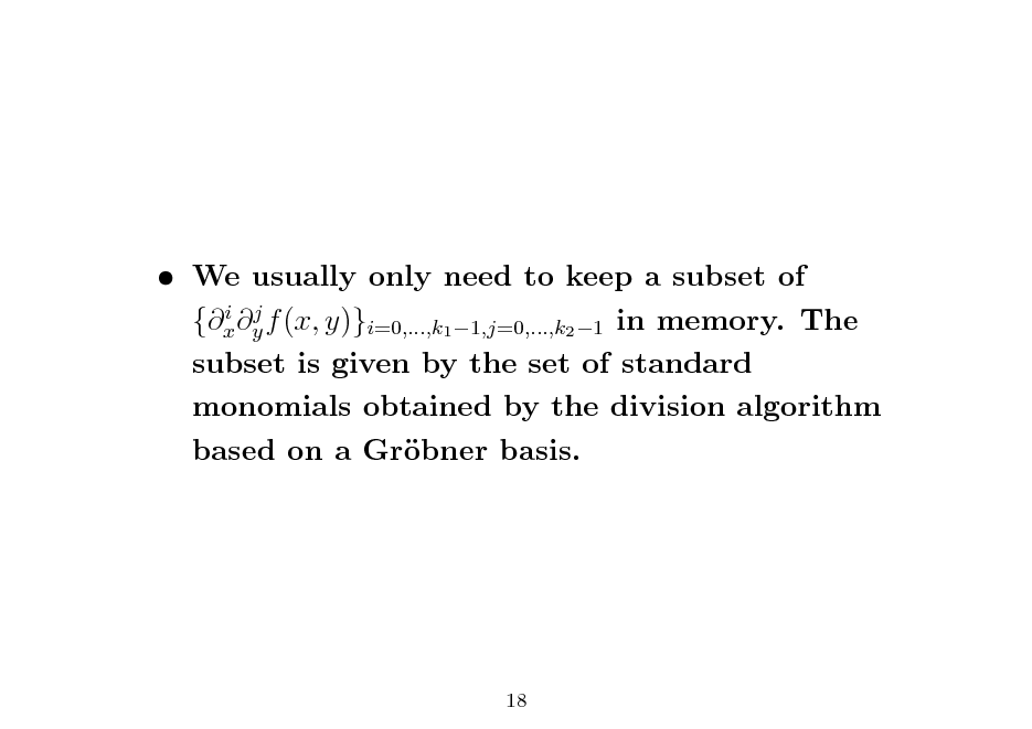
We usually only need to keep a subset of i j {x y f (x, y)}i=0,...,k1 1,j=0,...,k2 1 in memory. The subset is given by the set of standard monomials obtained by the division algorithm based on a Grbner basis. o

18

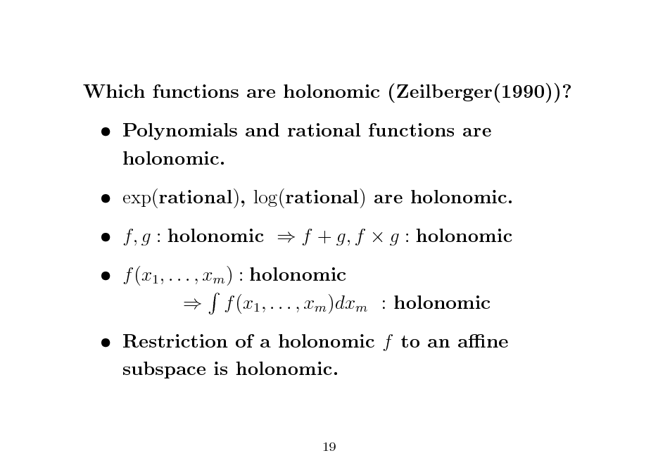
Which functions are holonomic (Zeilberger(1990))? Polynomials and rational functions are holonomic. exp(rational), log(rational) are holonomic. f, g : holonomic f + g, f g : holonomic f (x1 , . . . , xm ) : holonomic f (x1 , . . . , xm )dxm : holonomic Restriction of a holonomic f to an ane subspace is holonomic.

19

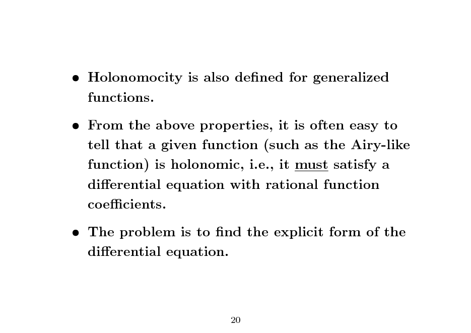
Holonomocity is also dened for generalized functions. From the above properties, it is often easy to tell that a given function (such as the Airy-like function) is holonomic, i.e., it must satisfy a dierential equation with rational function coecients. The problem is to nd the explicit form of the dierential equation.

20

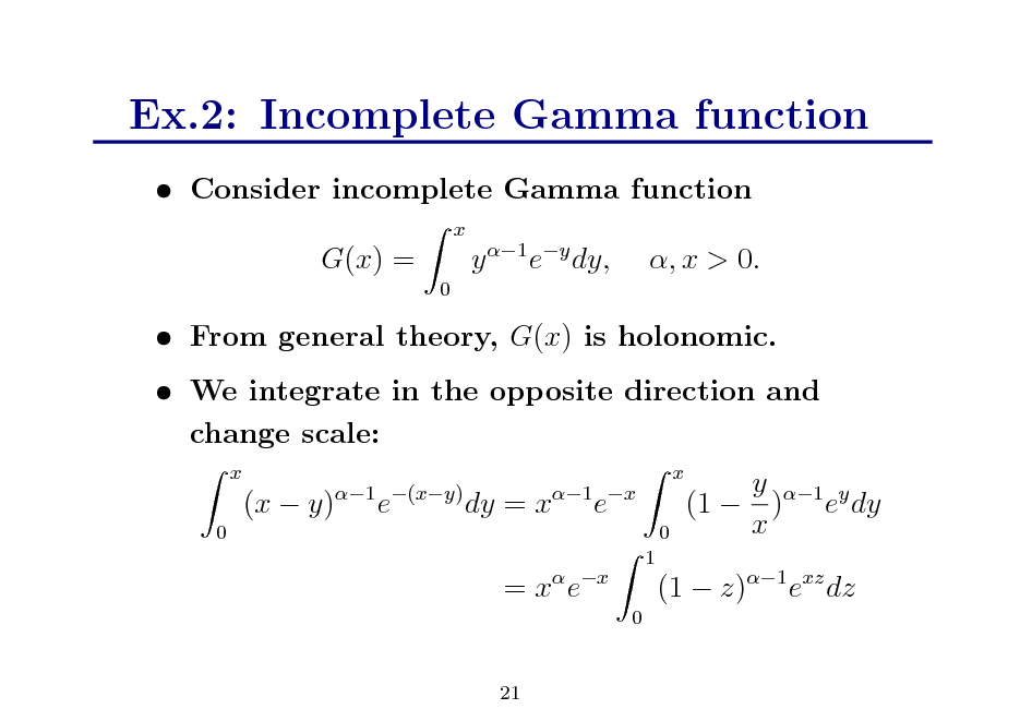
Ex.2: Incomplete Gamma function
Consider incomplete Gamma function
x

G(x) =
0

y 1 ey dy,

, x > 0.

From general theory, G(x) is holonomic. We integrate in the opposite direction and change scale:
x 0

(x y)

1 (xy)

e

dy = x

1 x

x 0

e

y 1 y (1 ) e dy x

= x ex
0

1

(1 z)1 exz dz

21

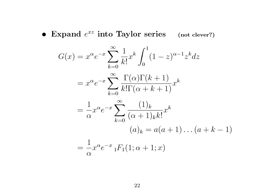
Expand exz into Taylor series G(x) = x ex =x e
x k=0

(not clever?)

1 k x k!

1 0

(1 z)1 z k dz

1 = x e

k=0 x

()(k + 1) k x k!( + k + 1) (1)k xk ( + 1)k k! (a)k = a(a + 1) . . . (a + k 1)

k=0

1 x = x e 1F1 (1; + 1; x)

22

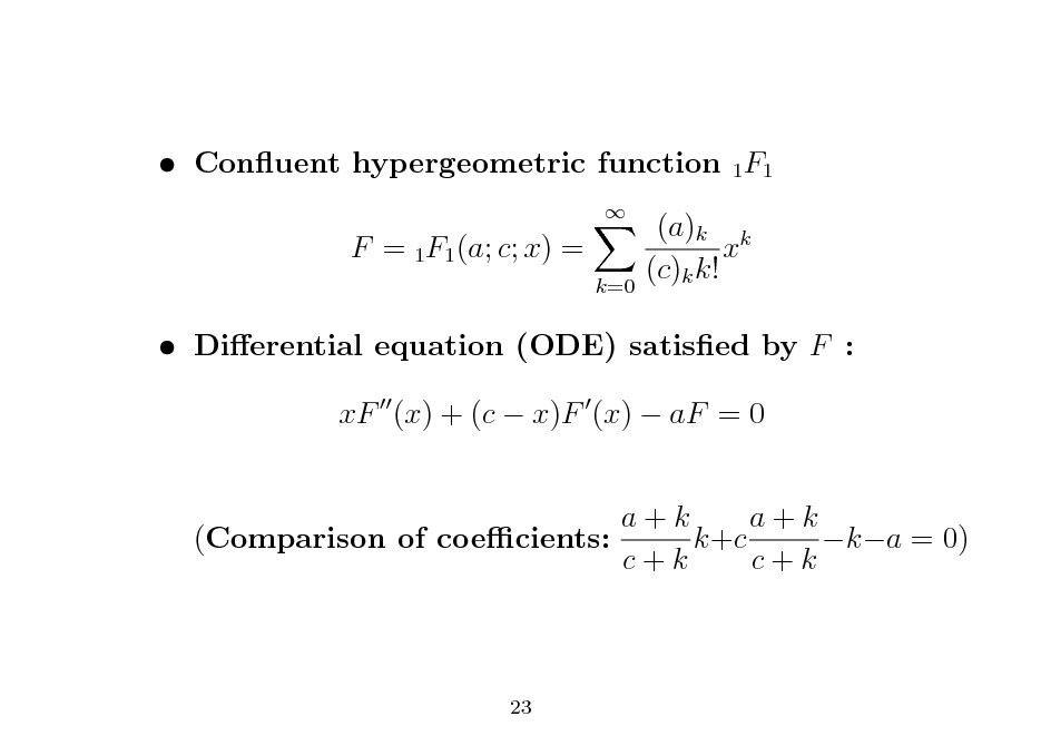
Conuent hypergeometric function 1F1 F = 1F1 (a; c; x) =
k=0

(a)k k x (c)k k!

Dierential equation (ODE) satised by F : xF (x) + (c x)F (x) aF = 0 a+k a+k (Comparison of coecients: k+c ka = 0) c+k c+k

23

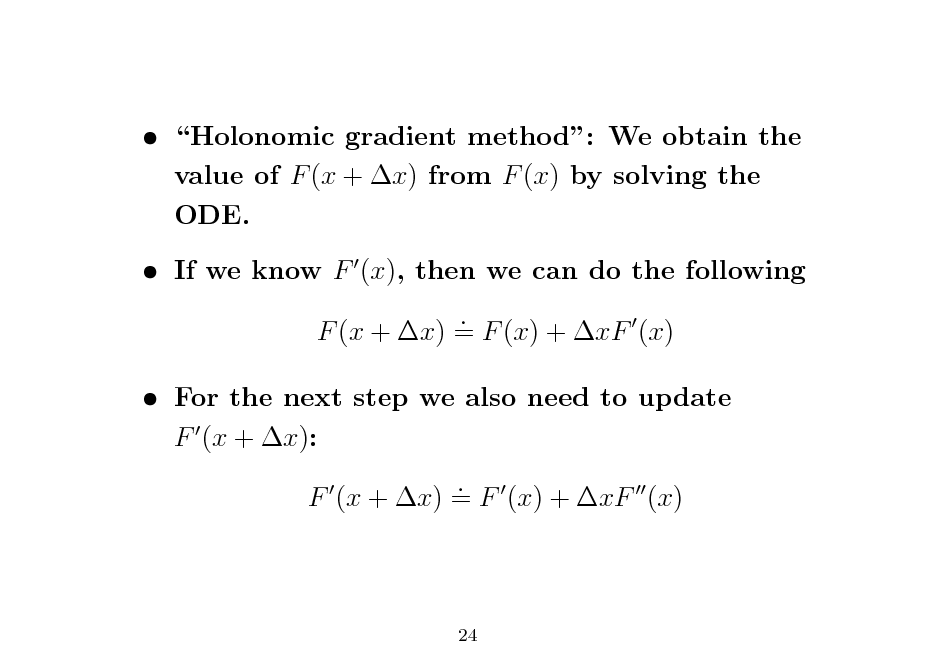
Holonomic gradient method: We obtain the value of F (x + x) from F (x) by solving the ODE. If we know F (x), then we can do the following . F (x + x) = F (x) + xF (x)

For the next step we also need to update F (x + x): . F (x + x) = F (x) + xF (x)

24

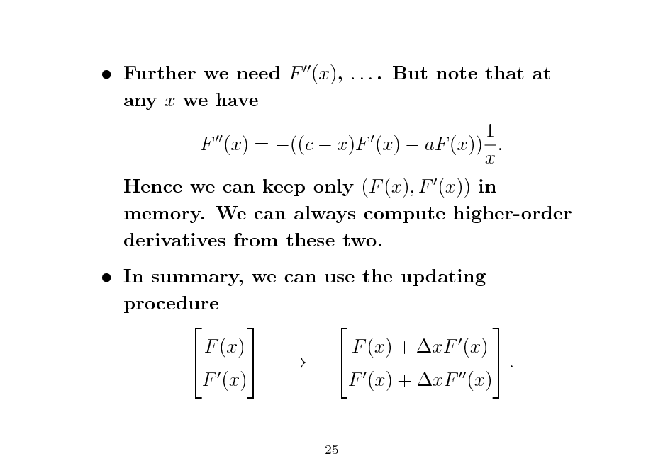
Further we need F (x), . . . . But note that at any x we have 1 F (x) = ((c x)F (x) aF (x)) . x Hence we can keep only (F (x), F (x)) in memory. We can always compute higher-order derivatives from these two. In summary, we can use the updating procedure F (x) F (x) + xF (x) . F (x) F (x) + xF (x)
25

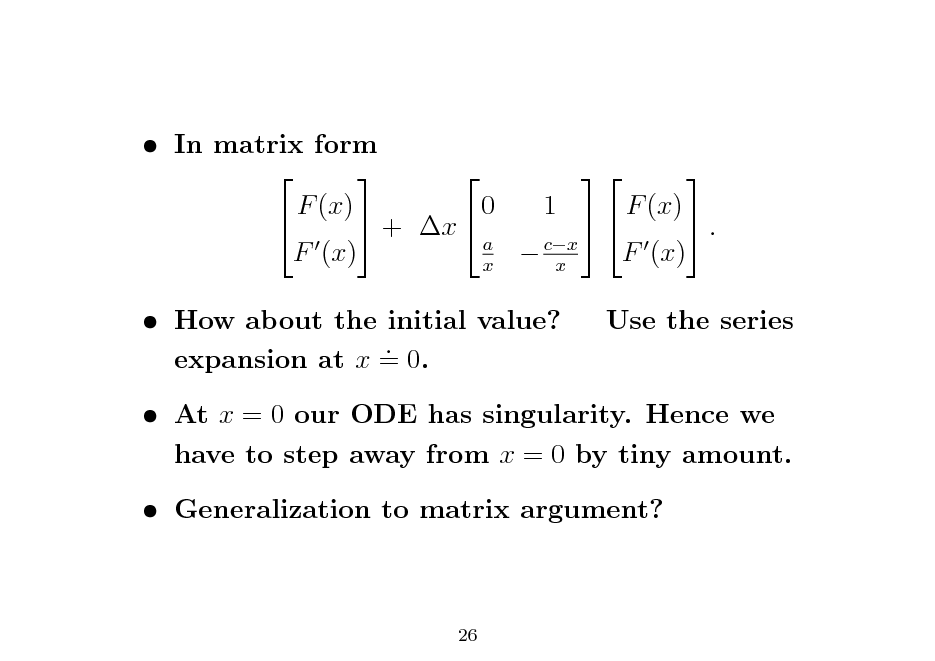
In matrix form F (x) 0 1 F (x) + x . a F (x) cx F (x) x x How about the initial value? . expansion at x = 0.

Use the series

At x = 0 our ODE has singularity. Hence we have to step away from x = 0 by tiny amount. Generalization to matrix argument?

26

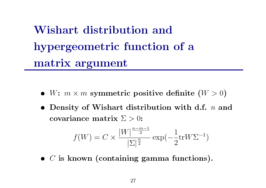
Wishart distribution and hypergeometric function of a matrix argument
W : m m symmetric positive denite (W > 0) Density of Wishart distribution with d.f. n and covariance matrix > 0: |W | f (W ) = C n || 2
nm1 2

1 exp( trW 1 ) 2

C is known (containing gamma functions).
27

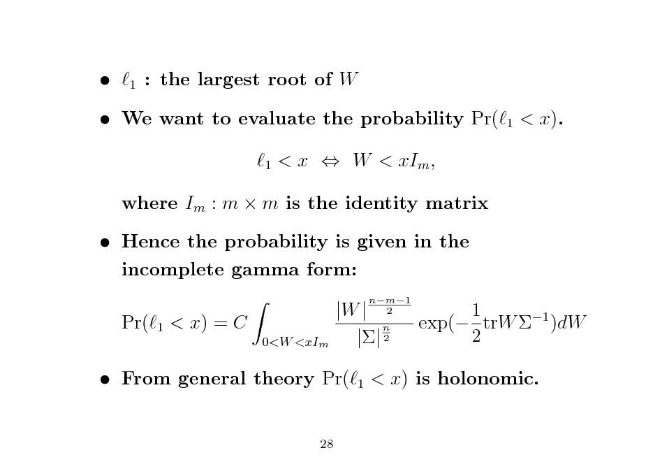
1

: the largest root of W
1

We want to evaluate the probability Pr(
1

< x).

< x W < xIm ,

where Im : m m is the identity matrix Hence the probability is given in the incomplete gamma form: Pr(
1

< x) = C
0<W <xIm

|W | n || 2
1

nm1 2

1 exp( trW 1 )dW 2

From general theory Pr(
28

< x) is holonomic.

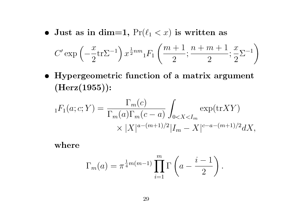
Just as in dim=1, Pr(

1

< x) is written as m + 1 n + m + 1 x 1 ; ; 2 2 2

1 x 1 C exp tr x 2 nm 1F1 2

Hypergeometric function of a matrix argument (Herz(1955)): m (c) 1F1 (a; c; Y ) = m (a)m (c a) where m (a) =
1 m(m1) 4

exp(trXY )
0<X<Im

|X|a(m+1)/2 |Im X|ca(m+1)/2 dX, i1 a 2 i=1
m

.

29

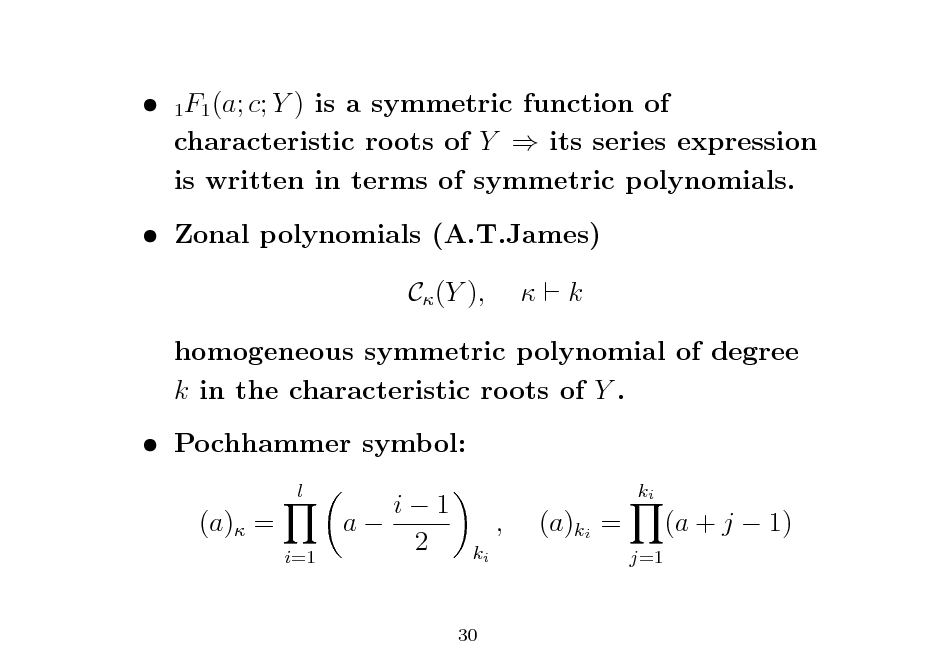
1F1 (a; c; Y ) is a symmetric function of characteristic roots of Y its series expression is written in terms of symmetric polynomials. Zonal polynomials (A.T.James) C (Y ), k

homogeneous symmetric polynomial of degree k in the characteristic roots of Y . Pochhammer symbol:
l

(a) =
i=1

i1 a 2

ki

,
ki

(a)ki =
j=1

(a + j 1)

30

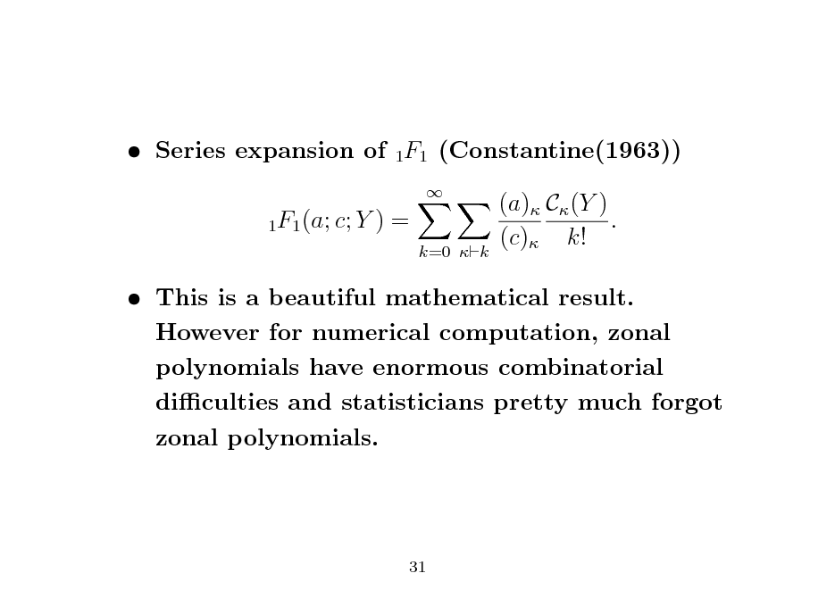
Series expansion of 1F1 (Constantine(1963))
1F1 (a; c; Y

)=

k=0 k

(a) C (Y ) . (c) k!

This is a beautiful mathematical result. However for numerical computation, zonal polynomials have enormous combinatorial diculties and statisticians pretty much forgot zonal polynomials.

31

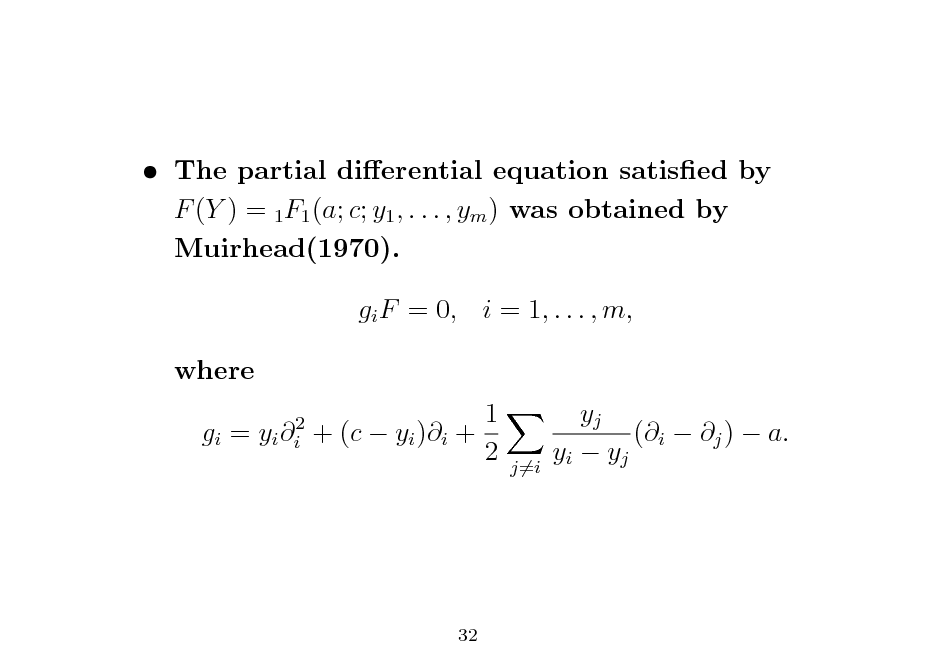
The partial dierential equation satised by F (Y ) = 1F1 (a; c; y1 , . . . , ym ) was obtained by Muirhead(1970). gi F = 0, i = 1, . . . , m, where gi = yi i2 1 + (c yi )i + 2 yj (i j ) a. yi yj

j=i

32

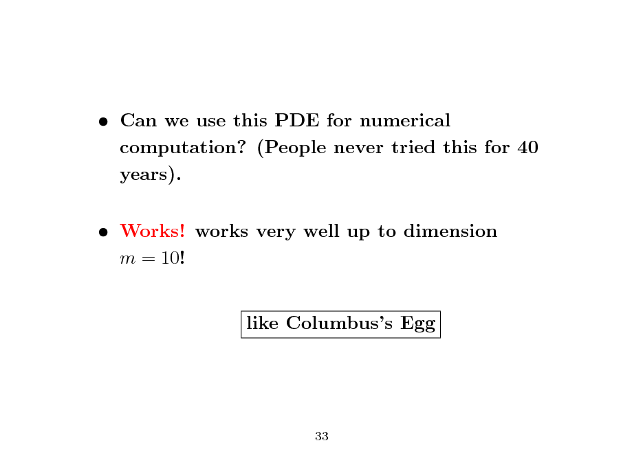
Can we use this PDE for numerical computation? (People never tried this for 40 years). Works! works very well up to dimension m = 10! like Columbuss Egg

33

Holonomic gradient method for dimension two
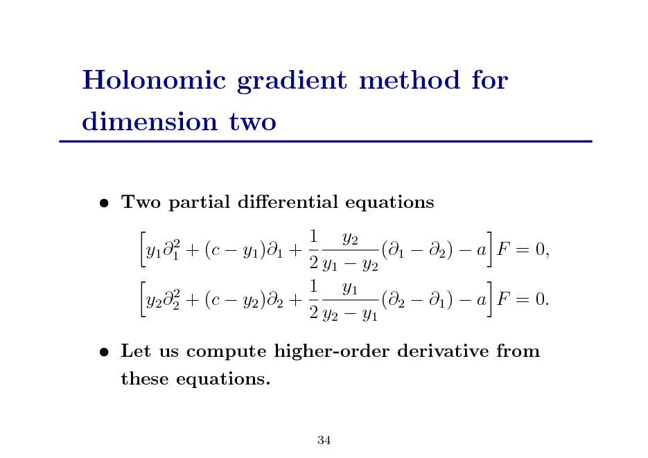
Two partial dierential equations 1 y2 + (c y1 )1 + (1 2 ) a F = 0, 2 y1 y2 1 y1 2 y2 2 + (c y2 )2 + (2 1 ) a F = 0. 2 y2 y1
2 y1 1

Let us compute higher-order derivative from these equations.
34

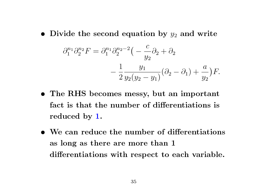
Divide the second equation by y2 and write
n n 1 1 2 2 F

=

n n 1 1 2 2 2

c 2 + 2 y2 1 y1 a (2 1 ) + F. 2 y2 (y2 y1 ) y2

The RHS becomes messy, but an important fact is that the number of dierentiations is reduced by 1. We can reduce the number of dierentiations as long as there are more than 1 dierentiations with respect to each variable.

35

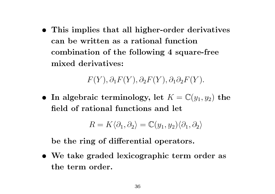
This implies that all higher-order derivatives can be written as a rational function combination of the following 4 square-free mixed derivatives: F (Y ), 1 F (Y ), 2 F (Y ), 1 2 F (Y ). In algebraic terminology, let K = C(y1 , y2 ) the eld of rational functions and let R = K 1 , 2 = C(y1 , y2 ) 1 , 2 be the ring of dierential operators. We take graded lexicographic term order as the term order.
36

Theorem 1 {g1 , g2 } is a Grbner basis and o {1, 1 , 2 , 1 2 } is the set of standard monomials. (This theorem hold for general dimension.) [Division algorithm] by repeating the dierentiations, for each n1 , n2 there exist (n ,n ) (n ,n ) (n ,n ) (n ,n ) rational functions h001 2 , h101 2 , h011 2 , h111 2 in y1 , y2 , such that
n n 1 1 2 2 F = h001 (n ,n2 )

F + h101

(n ,n2 )

1 F + h011

(n ,n2 )

2 F

+ h111

(n ,n2 )

1 2 F.

37

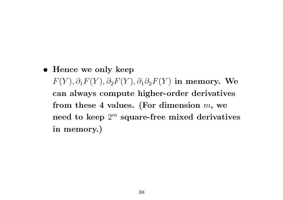
Hence we only keep F (Y ), 1 F (Y ), 2 F (Y ), 1 2 F (Y ) in memory. We can always compute higher-order derivatives from these 4 values. (For dimension m, we need to keep 2m square-free mixed derivatives in memory.)

38

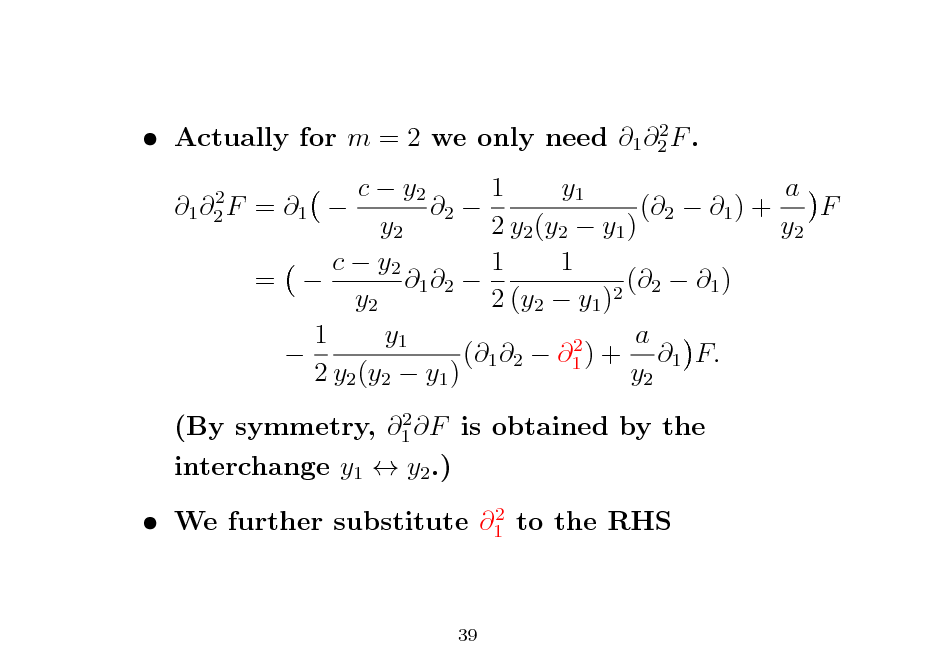
2 Actually for m = 2 we only need 1 2 F . 2 1 2 F

c y2 1 y1 a = 1 2 (2 1 ) + F y2 2 y2 (y2 y1 ) y2 c y2 1 1 = 1 2 (2 1 ) 2 y2 2 (y2 y1 ) 1 y1 a 2 (1 2 1 ) + 1 F. 2 y2 (y2 y1 ) y2

2 (By symmetry, 1 F is obtained by the interchange y1 y2 .) 2 We further substitute 1 to the RHS

39

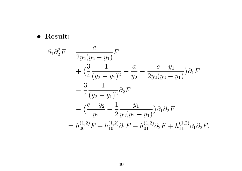
Result:
2 1 2 F

=

a

= h00 F + h10 1 F + h01 2 F + h11 1 2 F.

2y2 (y2 y1 ) 3 1 a c y1 + + 1 F 2 4 (y2 y1 ) y2 2y2 (y2 y1 ) 3 1 F 2 2 4 (y2 y1 ) c y2 1 y1 + 1 2 F y2 2 y2 (y2 y1 )
(1,2) (1,2) (1,2) (1,2)

F

40

Then as in the one-dimensional case, we can update: F (y1 + y1 , y2 + y2 ) . = F (y1 , y2 ) + y1 1 F (y1 , y2 ) + y2 2 F (y1 , y2 ), 1 F (y1 + y1 , y2 + y2 ) . 2 = 1 F (y1 , y2 ) + y1 1 F (y1 , y2 ) + y2 1 2 F (y1 , y2 ), [2 F is similar] 1 2 F (y1 + y1 , y2 + y2 ) . 2 2 = 1 2 F (y1 , y2 ) + y1 1 2 F (y1 , y2 ) + y2 1 2 F (y1 , y2 ).

41

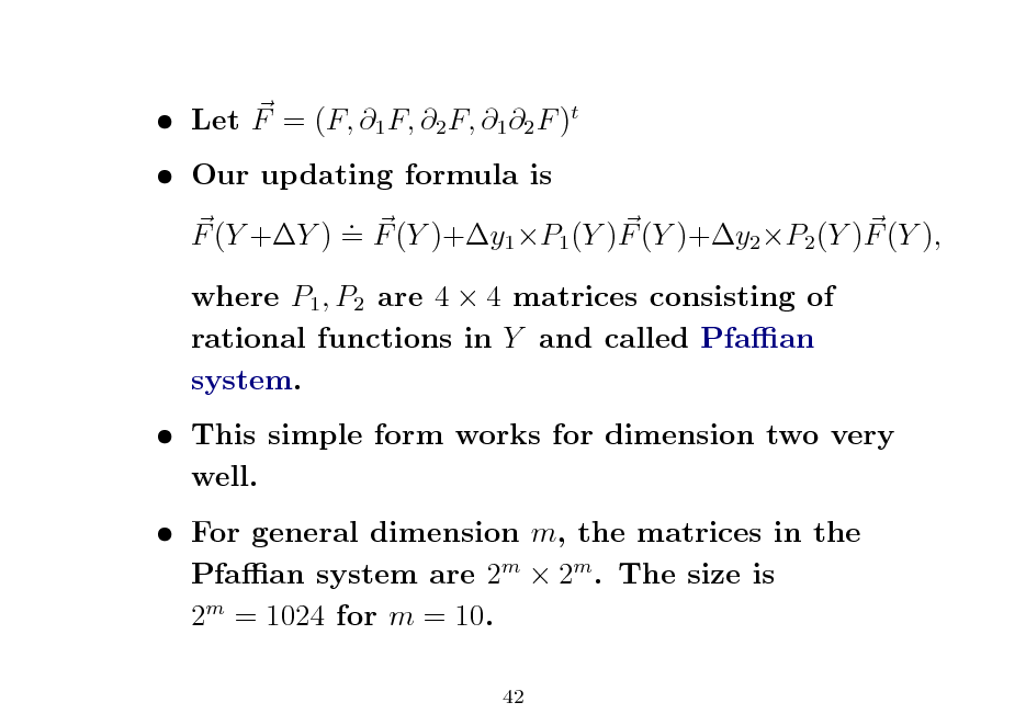
Let F = (F, 1 F, 2 F, 1 2 F )t Our updating formula is . F (Y +Y ) = F (Y )+y1 P1 (Y )F (Y )+y2 P2 (Y )F (Y ), where P1 , P2 are 4 4 matrices consisting of rational functions in Y and called Pfaan system. This simple form works for dimension two very well. For general dimension m, the matrices in the Pfaan system are 2m 2m . The size is 2m = 1024 for m = 10.
42

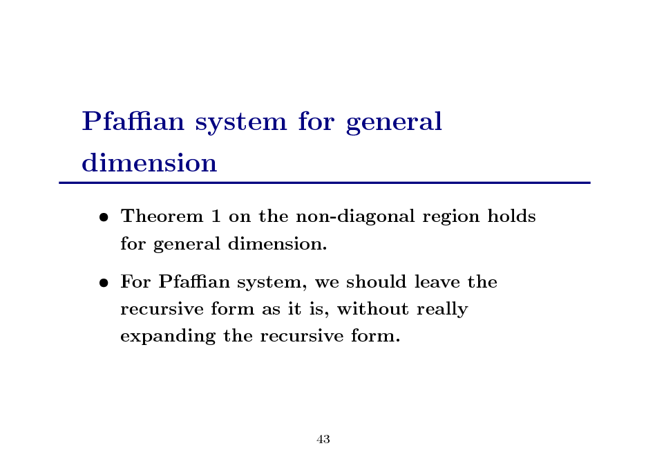
Pfaan system for general dimension
Theorem 1 on the non-diagonal region holds for general dimension. For Pfaan system, we should leave the recursive form as it is, without really expanding the recursive form.

43

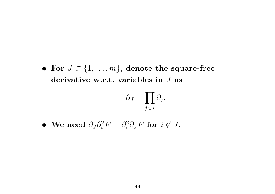
For J {1, . . . , m}, denote the square-free derivative w.r.t. variables in J as J =
jJ

j .

We need J i2 F = i2 J F for i J.

44

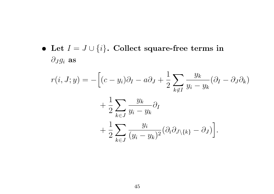
Let I = J {i}. Collect square-free terms in J gi as 1 r(i, J; y) = (c yi )I aJ + 2 1 + 2 1 + 2 yk I yi yk yk (I J k ) yi yk

kI

kJ

kJ

yi (i J\{k} J ) . 2 (yi yk )

45

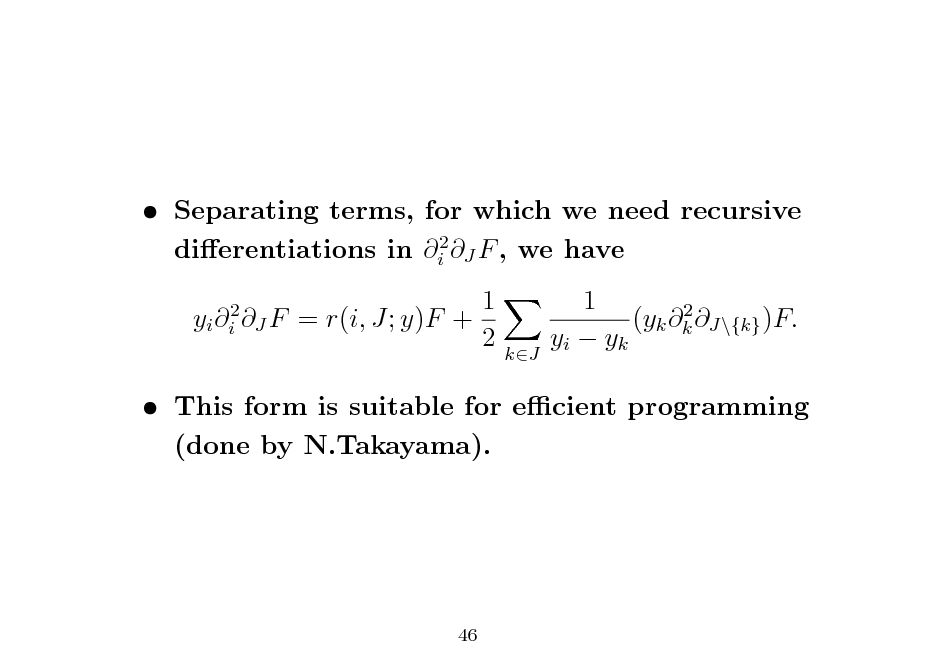
Separating terms, for which we need recursive dierentiations in i2 J F , we have yi i2 J F 1 = r(i, J; y)F + 2 1 2 (yk k J\{k} )F. yi yk

kJ

This form is suitable for ecient programming (done by N.Takayama).

46

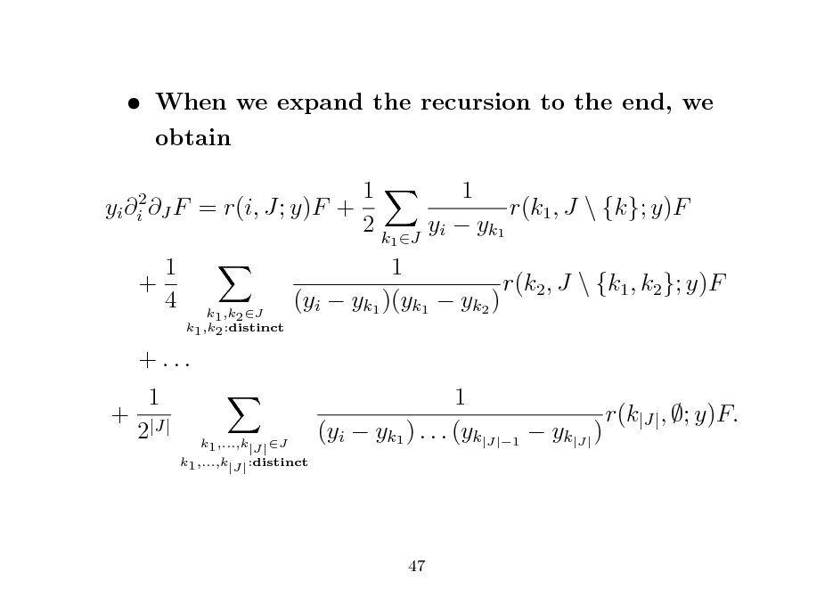
When we expand the recursion to the end, we obtain yi i2 J F 1 + 4 1 = r(i, J; y)F + 2k 1 r(k1 , J \ {k}; y)F y i y k1

k1 ,k2 J k1 ,k2 :distinct

1 r(k2 , J \ {k1 , k2 }; y)F (yi yk1 )(yk1 yk2 ) 1 r(k|J| , ; y)F. (yi yk1 ) . . . (yk|J|1 yk|J| )

1 J

+ ... 1 + |J| 2

k1 ,...,k|J| :distinct

k1 ,...,k|J| J

47

This form is also useful for theoretical consideration of the Pfaan system. The problem of initial values is also dicult in general dimension. N.Takayama expanded the algorithm of Koev-Edelman(2006) to handle partial derivatives.

48

Numerical experiments
Statisticians need good numerical performance (recall zonal polynomials). We were not sure whether it works up to dimension m = 10. How can we check the numerical accuracy? The initial value is taken to be close to zero. We can check the numerical convergence limx Pr( 1 < x) = 1.

49

The following easy bounds are available: Pr[
1 2 2 < x|diag(1 , . . . , 1 )]

Pr[

1

2 2 < x|diag(1 , . . . , m )] 1 2 < x|diag(1 , 0, . . . , 0)].

Pr[

Example: m = 10, d.f. n = 12, 1 = 2 diag(1, 2, . . . , 10).

50

For x = 30 the bounds are (0.99866943, 0.99999998). Intel Core i7 machine. The computation of the initial value at x0 = 0.2 takes 20 seconds. Then with the step size 0.001, we solve the PDE up to x = 30, which takes 75 seconds. Output: Pr[
1

< 30] = 0.999545

This accuracy is somewhat amazing, if we consider that we updated a 1024-dimensional vector 30,000 times.

51

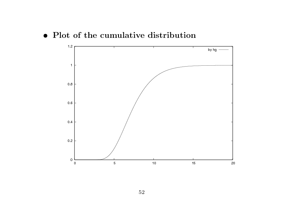
Plot of the cumulative distribution
1.2 by hg 1

0.8

0.6

0.4

0.2

0

0

5

10

15

20

52

Summary
Holonomic gradient method is practical if we implement it eciently. Our approach brought a totally new approach to a longstanding dicult problem in multivariate statistics. Holonomic gradient methods is general and can be applied to many problems. We stand at the beginning of applications of D-module theory to statistics!
53