
Machine Learning Summer School Kyoto 2012
Graph Mining
Chapter 1: Data Mining
National Institute of Advanced Industrial Science and Technology Koji Tsuda
1
Labeled graphs are general and powerful data structures that can be used to represent diverse kinds of objects such as XML code, chemical compounds, proteins, and RNAs. In these 10 years, we saw significant progress in statistical learning algorithms for graph data, such as supervised classification, clustering and dimensionality reduction. Graph kernels and graph mining have been the main driving force of such innovations. In this lecture, I start from basics of the two techniques and cover several important algorithms in learning from graphs. Successful biological applications are featured. If time allows, I will also cover recent developments and show future directions.
Scroll with j/k | | | Size

Machine Learning Summer School Kyoto 2012
Graph Mining
Chapter 1: Data Mining
National Institute of Advanced Industrial Science and Technology Koji Tsuda
1
1
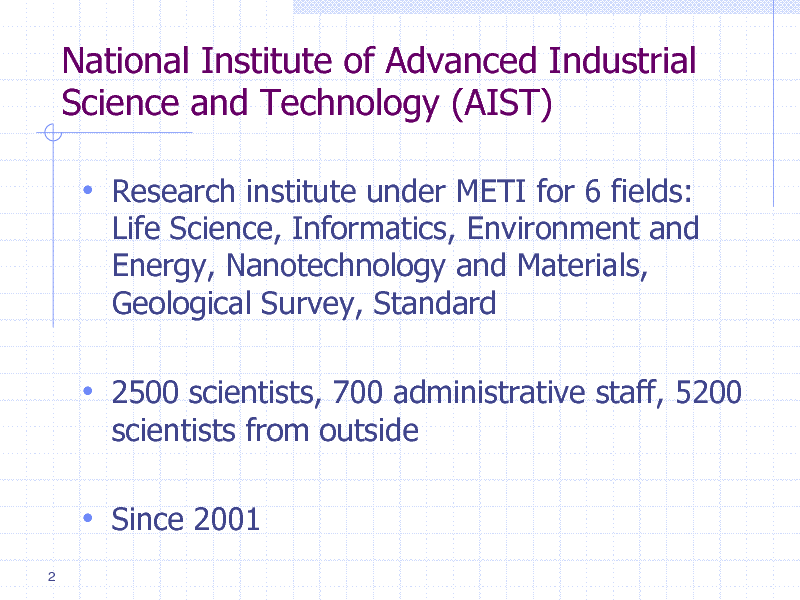
National Institute of Advanced Industrial Science and Technology (AIST)
Research institute under METI for 6 fields:
Life Science, Informatics, Environment and Energy, Nanotechnology and Materials, Geological Survey, Standard
2500 scientists, 700 administrative staff, 5200
scientists from outside
Since 2001
2
2

Computational Biology Research Center
Odaiba, Tokyo
Developing Novel Methods and Tools for
Genome Informatics Molecular Informatics Cellular Informatics
Diverse Collaboration with Companies and Universities
3
3
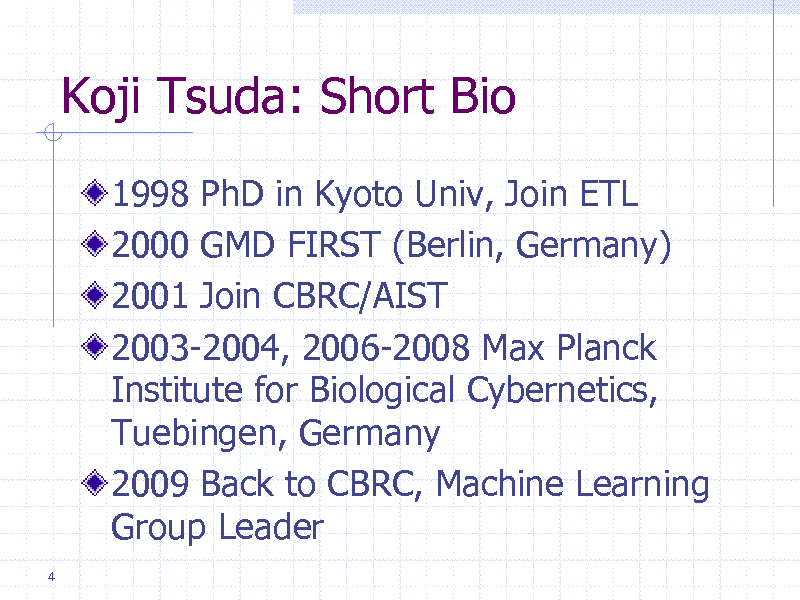
Koji Tsuda: Short Bio
1998 PhD in Kyoto Univ, Join ETL 2000 GMD FIRST (Berlin, Germany) 2001 Join CBRC/AIST 2003-2004, 2006-2008 Max Planck Institute for Biological Cybernetics, Tuebingen, Germany 2009 Back to CBRC, Machine Learning Group Leader
4
4
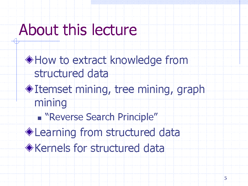
About this lecture
How to extract knowledge from structured data Itemset mining, tree mining, graph mining
Reverse Search Principle
Learning from structured data Kernels for structured data
5
5
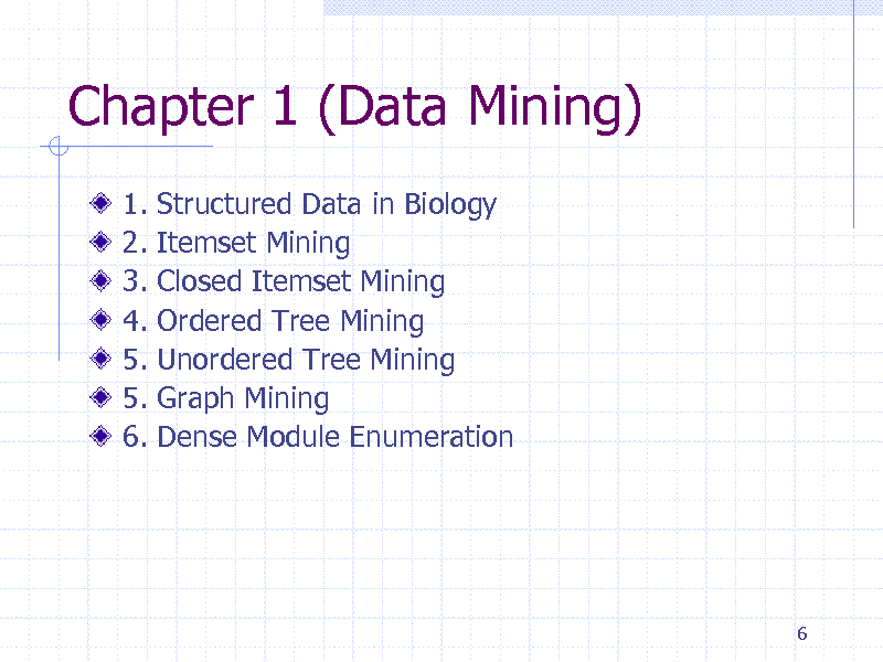
Chapter 1 (Data Mining)
1. 2. 3. 4. 5. 5. 6. Structured Data in Biology Itemset Mining Closed Itemset Mining Ordered Tree Mining Unordered Tree Mining Graph Mining Dense Module Enumeration
6
6

Agenda 2 (Learning from Structured Data)
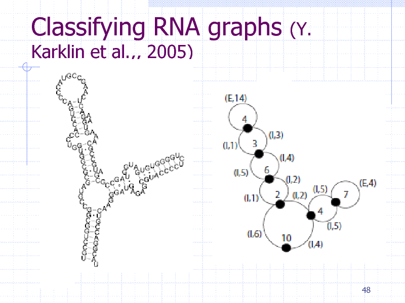
1. 2. 3. 4. 5. Preliminaries Graph Clustering by EM Graph Boosting Regularization Paths in Graph Classification Itemset Boosting for predicting HIV drug resistance
7
7
Agenda 3 (Kernel)
1. 2. 3. 4. 5. 6. Kernel Method Revisited Marginalized Kernels (Fisher Kernels) Marginalized Graph Kernels Weisfeiler-Lehman kernels Reaction Graph kernels Concluding Remark
8
8

Part 1: Structural Data in Biology
9
9
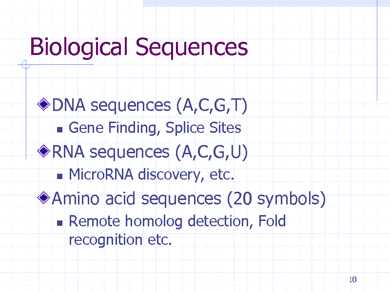
Biological Sequences
DNA sequences (A,C,G,T)
Gene Finding, Splice Sites MicroRNA discovery, etc. Remote homolog detection, Fold recognition etc.
10
RNA sequences (A,C,G,U)
Amino acid sequences (20 symbols)
10
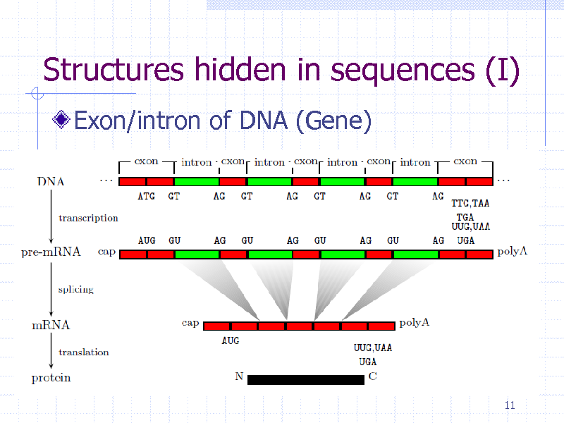
Structures hidden in sequences (I)
Exon/intron of DNA (Gene)
11
11
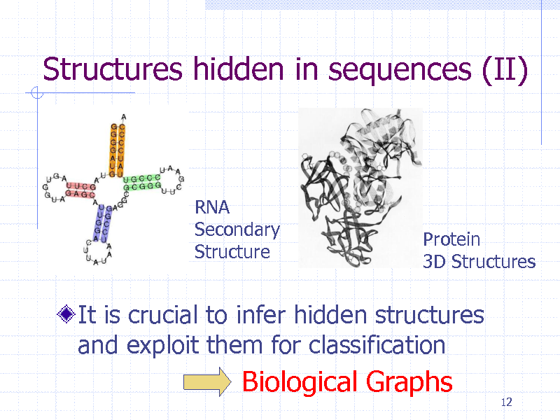
Structures hidden in sequences (II)
RNA Secondary Structure
Protein 3D Structures
It is crucial to infer hidden structures and exploit them for classification
Biological Graphs
12
12
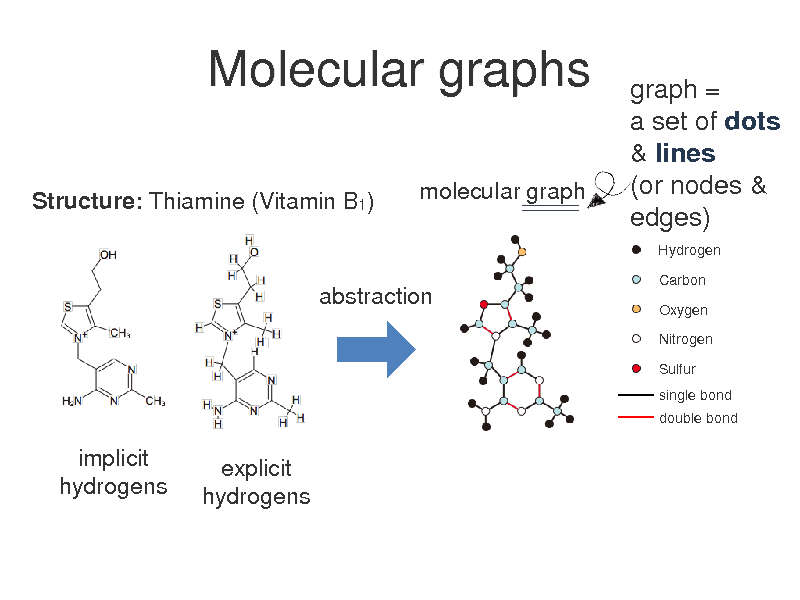
Molecular graphs
Structure: Thiamine (Vitamin B1) molecular graph
graph = a set of dots & lines (or nodes & edges)
Hydrogen Carbon Oxygen Nitrogen Sulfur single bond double bond
abstraction
implicit hydrogens
explicit hydrogens
13
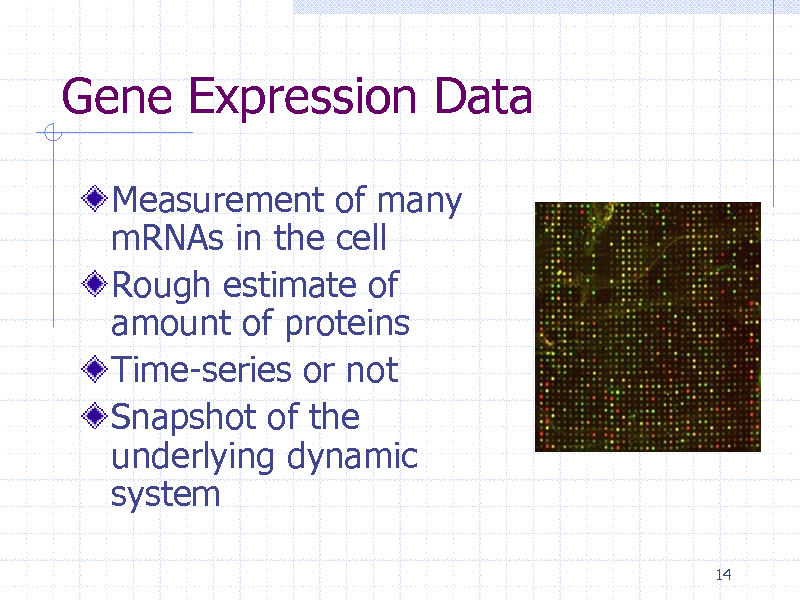
Gene Expression Data
Measurement of many mRNAs in the cell Rough estimate of amount of proteins Time-series or not Snapshot of the underlying dynamic system
14
14
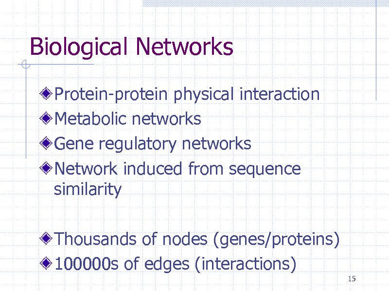
Biological Networks
Protein-protein physical interaction Metabolic networks Gene regulatory networks Network induced from sequence similarity
Thousands of nodes (genes/proteins) 100000s of edges (interactions)
15
15
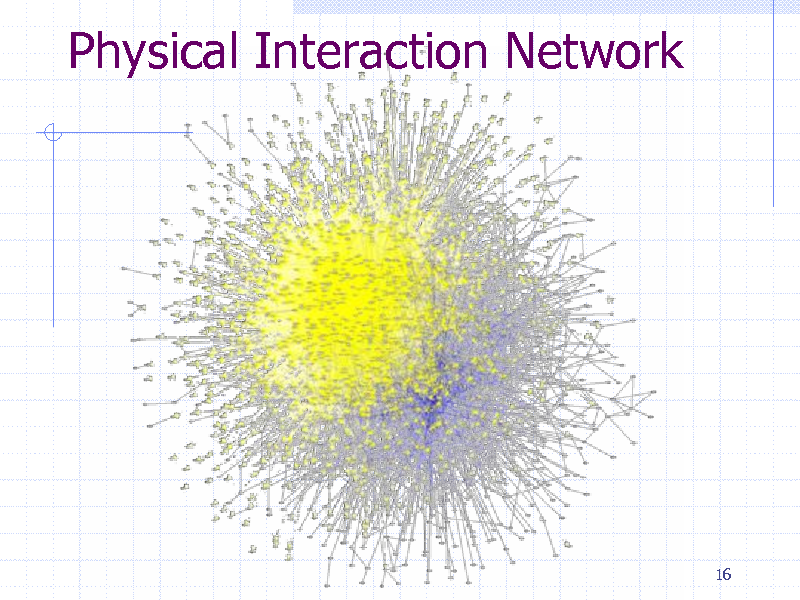
Physical Interaction Network
16
16
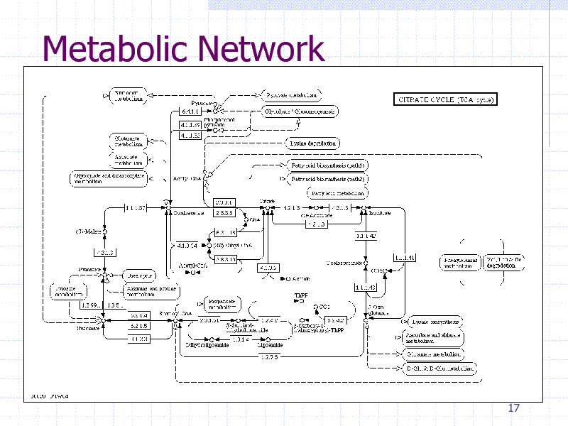
Metabolic Network
17
17
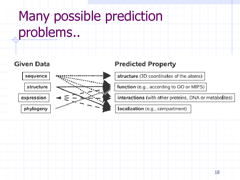
Many possible prediction problems..
18
18
Part 2: Itemset mining
19
19
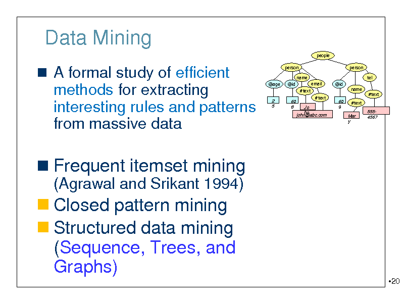
Data Mining
people
A formal study of efficient methods for extracting interesting rules and patterns
person name @age @id #text 2 5 60 8 #text Jo hn john@abc.com 60 9 email @id
person tel name #text Mar y
#text
from massive data
5554567
Frequent itemset mining
(Agrawal and Srikant 1994)
Closed pattern mining Structured data mining (Sequence, Trees, and Graphs)
20
20
![Slide: Frequent Itemset Mining
[Agrawal, Srikant, VLDB'94]
Finding all "frequent" sets of elements (items) appearing times or more in a database
Minsup = 2
1 t1 t2 t3 t4 t5 2 3 4 5
Frequent sets , 1, 2, 3, 4, 12, 13, 14, 23, 24, 124
X = {2, 4} appears three times, thus frequent
Frequent sets
21
database
The itemset lattice (2, )](https://yosinski.com/mlss12/media/slides/MLSS-2012-Tsuda-Graph-Mining_021.png)
Frequent Itemset Mining
[Agrawal, Srikant, VLDB'94]
Finding all "frequent" sets of elements (items) appearing times or more in a database
Minsup = 2
1 t1 t2 t3 t4 t5 2 3 4 5
Frequent sets , 1, 2, 3, 4, 12, 13, 14, 23, 24, 124
X = {2, 4} appears three times, thus frequent
Frequent sets
21
database
The itemset lattice (2, )
21
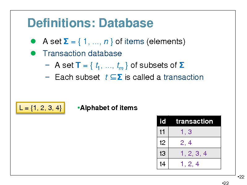
Definitions: Database
A set = { 1, ..., n } of items (elements) Transaction database A set T = { t1, ..., tm } of subsets of Each subset t is called a transaction
L = {1, 2, 3, 4}
Alphabet of items id t1 t2 t3 t4 transaction 1, 3 2, 4 1, 2, 3, 4 1, 2, 4
22 22
22
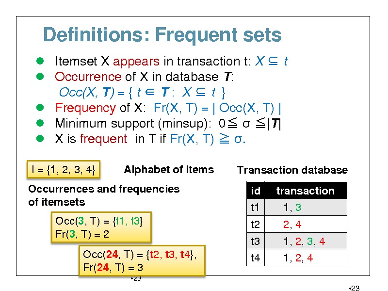
Definitions: Frequent sets
Itemset X appears in transaction t: X t Occurrence of X in database T: Occ(X, T) = { t T : X t } Frequency of X: Fr(X, T) = | Occ(X, T) | Minimum support (minsup): 0 |T| X is frequent in T if Fr(X, T) .
I = {1, 2, 3, 4} Alphabet of items Transaction database id t1 t2 t3 t4 transaction 1, 3 2, 4 1, 2, 3, 4 1, 2, 4
23
Occurrences and frequencies of itemsets Occ(3, T) = {t1, t3} Fr(3, T) = 2 Occ(24, T) = {t2, t3, t4}, Fr(24, T) = 3
23
23
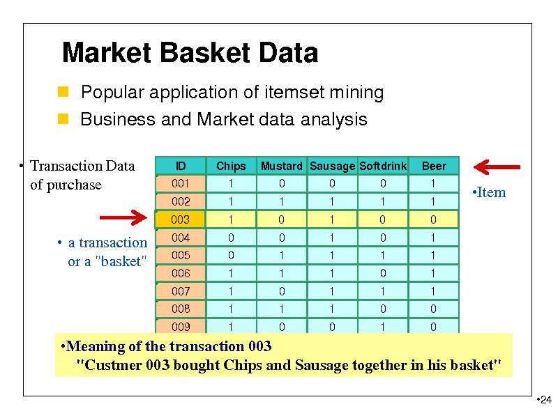
Market Basket Data
Popular application of itemset mining Business and Market data analysis
Transaction Data of purchase
ID 001 002 Chips 1 1 Mustard Sausage Softdrink 0 1 0 1 0 1 Beer 1 1
Item
003
1
0 0 1 1 1 1
0
0 1 1 0 1 0
1
1 1 1 1 1 0
0
0 1 0 1 0 1
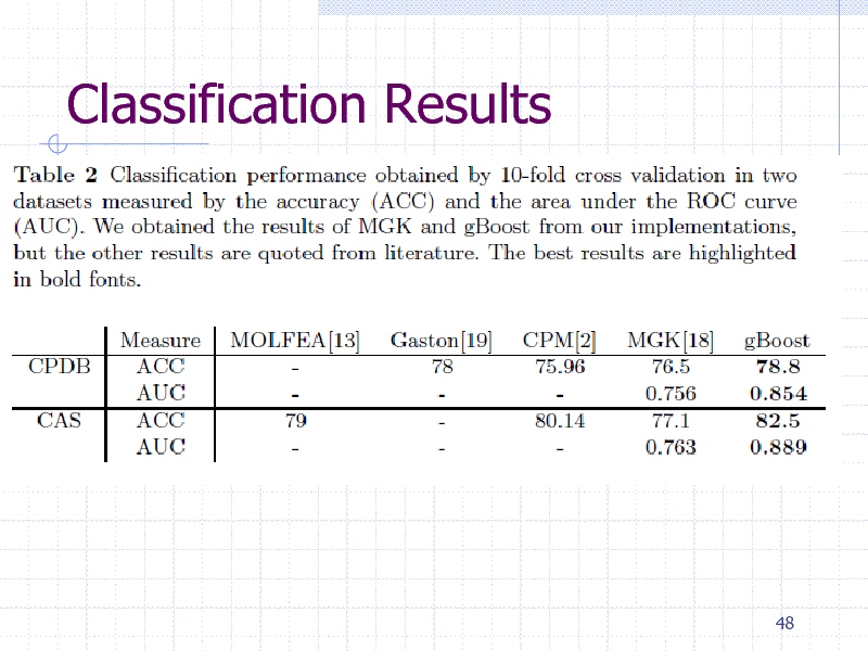
0
1 1 1 1 0 0
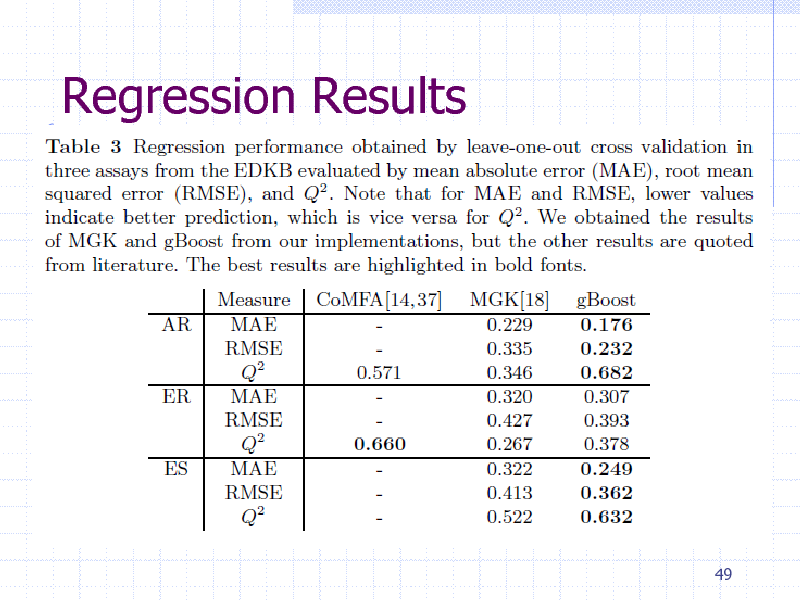
a transaction or a "basket"
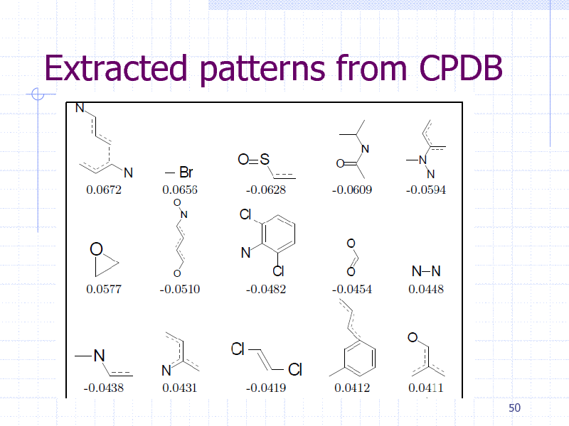
004 005 006 007 008 009
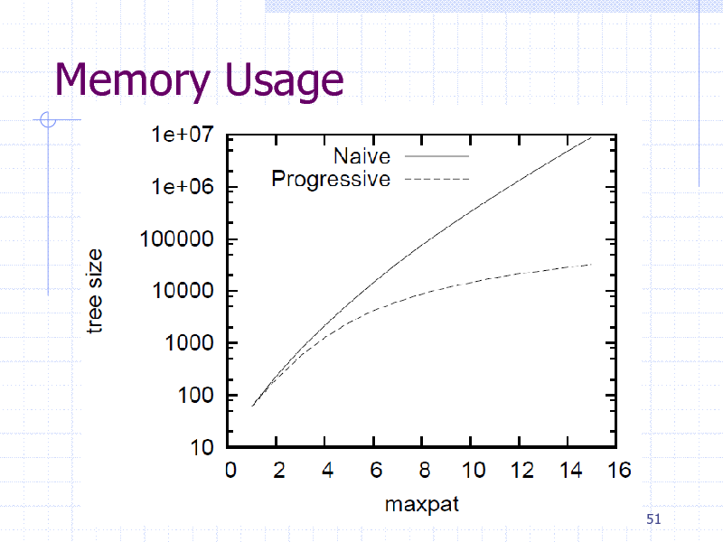
010 0 1 0 1 Meaning of the transaction 003 1 "Custmer 003 bought Chips and Sausage together in his basket"
24
24
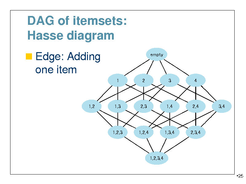
DAG of itemsets: Hasse diagram
Edge: Adding
empty
one item
1 2 3 4
1,2
1,3
2,3
1,4
2,4
3,4
1,2,3
1,2,4
1,3,4
2,3,4
1,2,3,4
25
25
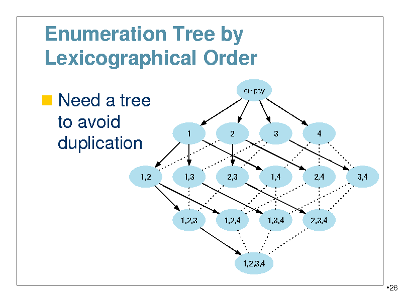
Enumeration Tree by Lexicographical Order
Need a tree
empty
to avoid duplication
1,2
1
2
3
4
1,3
2,3
1,4
2,4
3,4
1,2,3
1,2,4
1,3,4
2,3,4
1,2,3,4
26
26
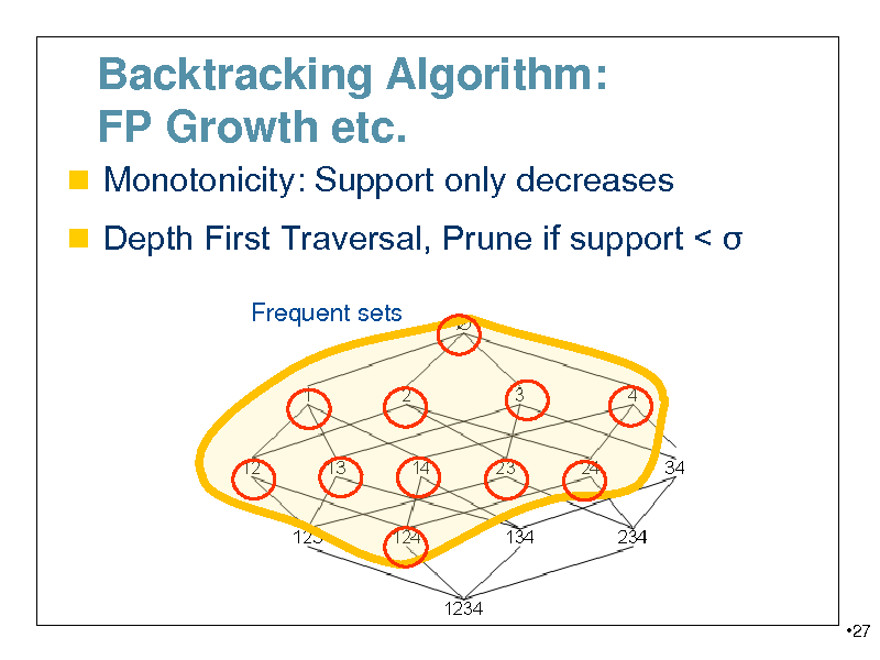
Backtracking Algorithm: FP Growth etc.
Monotonicity: Support only decreases Depth First Traversal, Prune if support <
Frequent sets
27
27
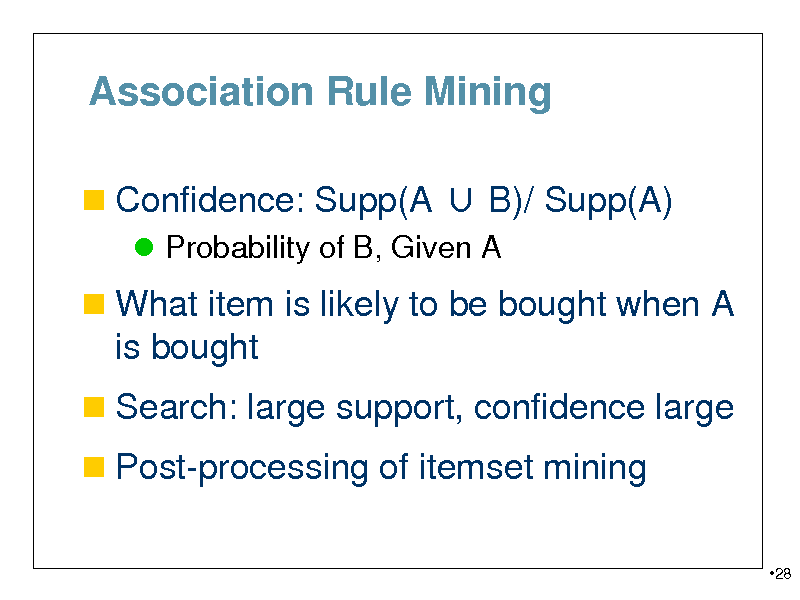
Association Rule Mining
Confidence: Supp(A B)/ Supp(A)
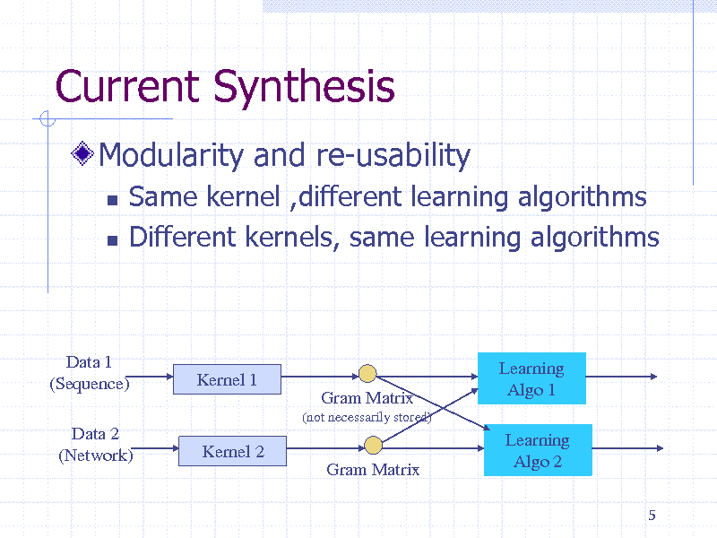
Probability of B, Given A
What item is likely to be bought when A
is bought
Search: large support, confidence large Post-processing of itemset mining
28
28
Summary: Itemset mining
Itemset mining is the simplest of all
mining algorithms
Need to maintain occurrence of each
pattern in database
Tree by lexicographical order is
(implicitly) used
29
29
Part 3: Closed Itemset mining
30
30
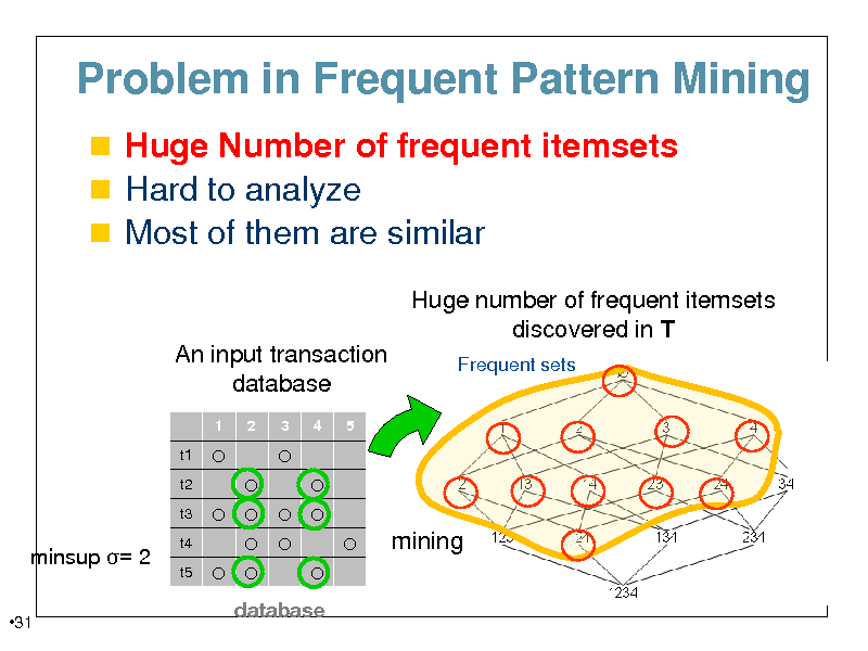
Problem in Frequent Pattern Mining
Huge Number of frequent itemsets Hard to analyze Most of them are similar
Huge number of frequent itemsets discovered in T
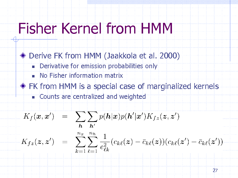
An input transaction database
1 t1 t2 t3 2 3 4 5
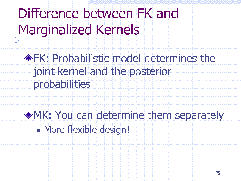
Frequent sets
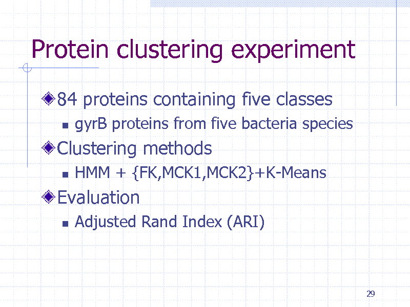
minsup = 2
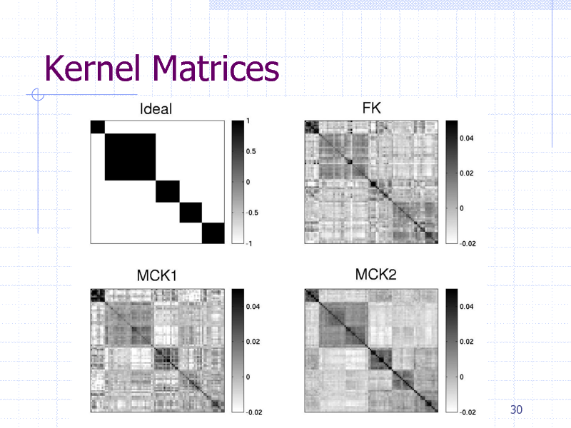
31
t4 t5
mining
database
31
![Slide: Solution: Closed Pattern Mining
Find only closed patterns Observation: Most frequent itemset X can be extended without changing occurrence by
adding new elements
def ([Pasquier et al., ICDT'99]). An itemset X is a closed set if and only if there is no proper superset of X with the same frequency (thus the same occurrence set).
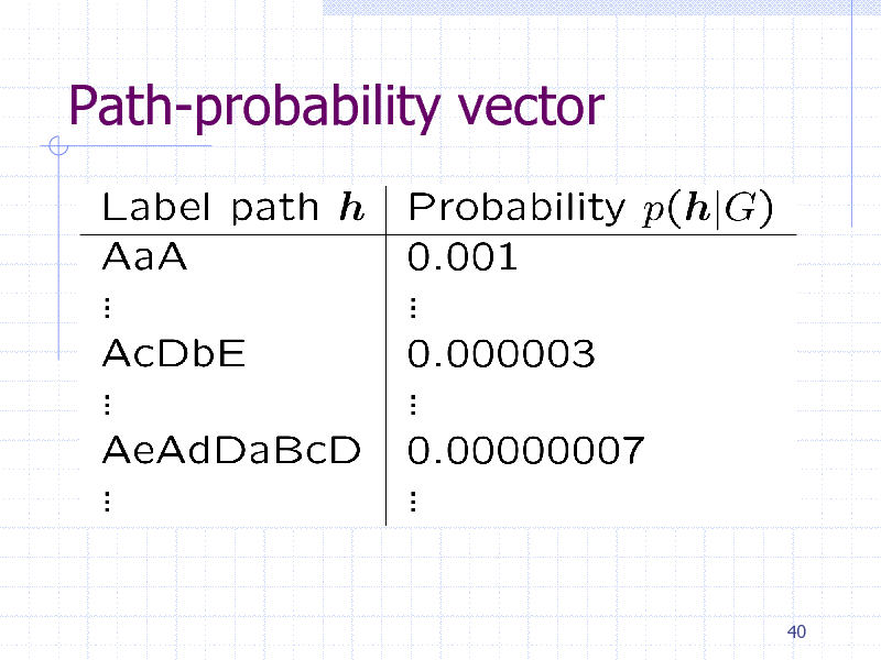
32](https://yosinski.com/mlss12/media/slides/MLSS-2012-Tsuda-Graph-Mining_032.png)
Solution: Closed Pattern Mining
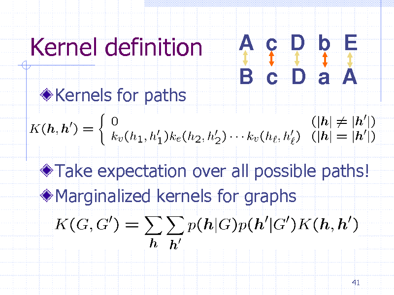
Find only closed patterns Observation: Most frequent itemset X can be extended without changing occurrence by
adding new elements
def ([Pasquier et al., ICDT'99]). An itemset X is a closed set if and only if there is no proper superset of X with the same frequency (thus the same occurrence set).
32
32
![Slide: Closed Pattern Mining
A closed itemset is the maximal set among all
itemsets with the same occurrences. Equivalence class [X] = {Y| Occ(X)=Occ(Y) }.
A AC AB ABC C AE ABE B BE ACE ABCE BC BCE E CE
Database
id 1 2 3 4 records ABCE AC BE BCE
Closed sets (maximal sets) Equivalence class w.r.t. occurrences
33](https://yosinski.com/mlss12/media/slides/MLSS-2012-Tsuda-Graph-Mining_033.png)
Closed Pattern Mining
A closed itemset is the maximal set among all
itemsets with the same occurrences. Equivalence class [X] = {Y| Occ(X)=Occ(Y) }.
A AC AB ABC C AE ABE B BE ACE ABCE BC BCE E CE
Database
id 1 2 3 4 records ABCE AC BE BCE
Closed sets (maximal sets) Equivalence class w.r.t. occurrences
33
33
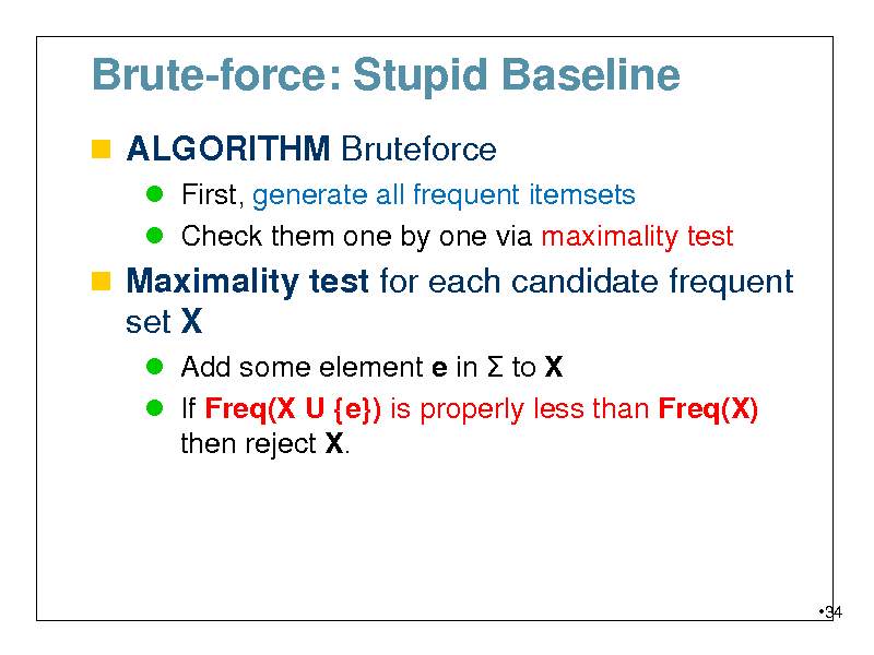
Brute-force: Stupid Baseline
ALGORITHM Bruteforce
First, generate all frequent itemsets Check them one by one via maximality test
Maximality test for each candidate frequent set X
Add some element e in to X If Freq(X U {e}) is properly less than Freq(X) then reject X.
34
34
![Slide: Bruteforce
STEP1) first, generate all frequent sets
Database T id 1 2 3 4
[1,2]
All itemsets in T
[1,2,4]
records ABCE AC BE BCE
[1,2,3,4] [1,3,4]
[1,2]
A AB ABC
C AE ABE
B BE ACE ABCE
[1]
E BC BCE
[1,4]
AC
CE
Occurrence (set of ids) Equivalence class w.r.t. occurrences Closed sets (maximal sets)
35](https://yosinski.com/mlss12/media/slides/MLSS-2012-Tsuda-Graph-Mining_035.png)
Bruteforce
STEP1) first, generate all frequent sets
Database T id 1 2 3 4
[1,2]
All itemsets in T
[1,2,4]
records ABCE AC BE BCE
[1,2,3,4] [1,3,4]
[1,2]
A AB ABC
C AE ABE
B BE ACE ABCE
[1]
E BC BCE
[1,4]
AC
CE
Occurrence (set of ids) Equivalence class w.r.t. occurrences Closed sets (maximal sets)
35
35
![Slide: Bruteforce
STEP1) first, generate all frequent sets STEP 2) make closedness test for each set
Database T id 1 2 3 4
[1,2]
All itemsets in T
[1,2,4]
records ABCE AC BE BCE
[1,2,3,4] [1,3,4]
[1,2]
A AB ABC
C AE ABE
B BE ACE ABCE
[1]
E BC BCE
[1,4]
AC
CE
Occurrence (set of ids) Equivalence class w.r.t. occurrences Closed sets (maximal sets)
36](https://yosinski.com/mlss12/media/slides/MLSS-2012-Tsuda-Graph-Mining_036.png)
Bruteforce
STEP1) first, generate all frequent sets STEP 2) make closedness test for each set
Database T id 1 2 3 4
[1,2]
All itemsets in T
[1,2,4]
records ABCE AC BE BCE
[1,2,3,4] [1,3,4]
[1,2]
A AB ABC
C AE ABE
B BE ACE ABCE
[1]
E BC BCE
[1,4]
AC
CE
Occurrence (set of ids) Equivalence class w.r.t. occurrences Closed sets (maximal sets)
36
36
![Slide: Bruteforce
STEP1) first, generate all frequent sets STEP 2) make closedness test for each set STEP3) finally, extract all closed sets
Database T id 1 2 3 4
[1,2]
All itemsets in T
[1,2,4]
records ABCE AC BE BCE
[1,2,3,4] [1,3,4]
[1,2]
A AB ABC
C AE ABE
B BE ACE ABCE
[1]
E BC BCE
[1,4]
AC
CE
Occurrence (set of ids) Equivalence class w.r.t. occurrences Closed sets (maximal sets)
All closed sets are found!
37](https://yosinski.com/mlss12/media/slides/MLSS-2012-Tsuda-Graph-Mining_037.png)
Bruteforce
STEP1) first, generate all frequent sets STEP 2) make closedness test for each set STEP3) finally, extract all closed sets
Database T id 1 2 3 4
[1,2]
All itemsets in T
[1,2,4]
records ABCE AC BE BCE
[1,2,3,4] [1,3,4]
[1,2]
A AB ABC
C AE ABE
B BE ACE ABCE
[1]
E BC BCE
[1,4]
AC
CE
Occurrence (set of ids) Equivalence class w.r.t. occurrences Closed sets (maximal sets)
All closed sets are found!
37
37
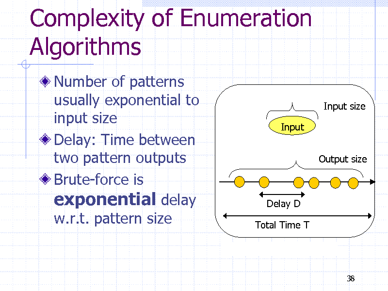
Complexity of Enumeration Algorithms
Number of patterns usually exponential to input size Delay: Time between two pattern outputs Brute-force is exponential delay w.r.t. pattern size
Input size Input Output size
Delay D Total Time T
38
38
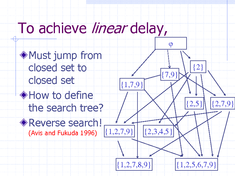
To achieve linear delay,
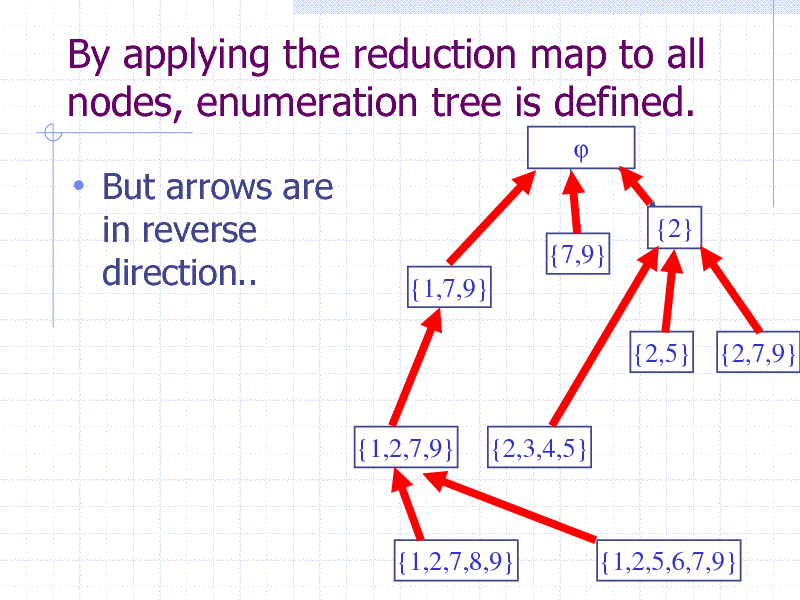
Must jump from closed set to closed set How to define the search tree? Reverse search!
(Avis and Fukuda 1996)
{2} {7,9} {1,7,9} {2,5} {2,7,9}
{1,2,7,9}
{2,3,4,5}
{1,2,7,8,9}
{1,2,5,6,7,9} 39
39
Reverse Search: Its a must
A general mathematical framework to design enumeration algorithms Can be used to prove the correctness of the algorithm Popular in computational geometry Data mining algorithms can be explained in remarkable simplicity
40
40
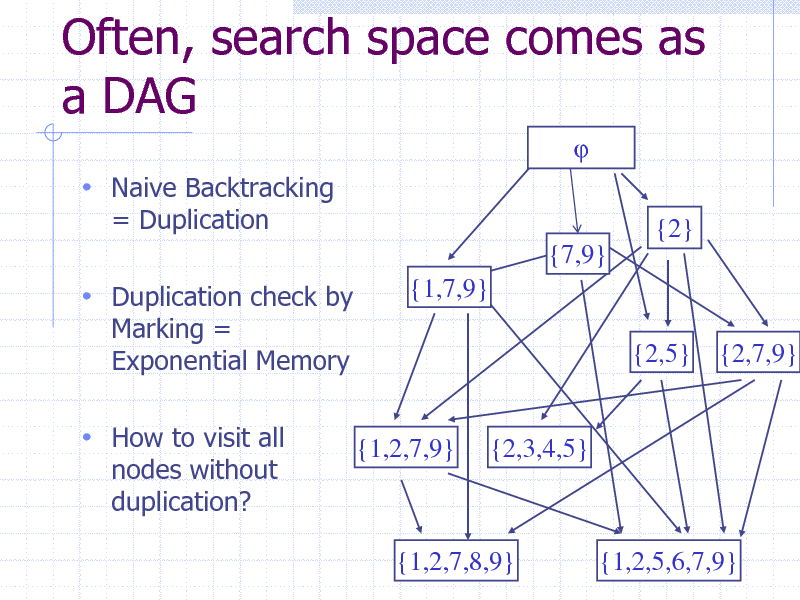
Often, search space comes as a DAG
Naive Backtracking
= Duplication {2} {7,9} {1,7,9} {2,5} {2,7,9}
Duplication check by
Marking = Exponential Memory
How to visit all
nodes without duplication?
{1,2,7,9}
{2,3,4,5}
{1,2,7,8,9}
{1,2,5,6,7,9} 41
41
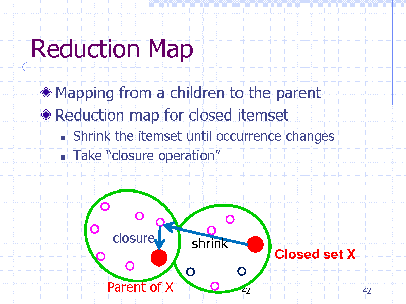
Reduction Map
Mapping from a children to the parent Reduction map for closed itemset
Shrink the itemset until occurrence changes Take closure operation
closure(X) closure shrink
Parent of X
42
Closed set X
42
42
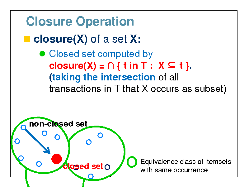
Closure Operation
closure(X) of a set X:
Closed set computed by closure(X) = { t in T : X t }. (taking the intersection of all transactions in T that X occurs as subset)
non-closed set
closure(X)
closed set
43
Equivalence class of itemsets with same occurrence
43
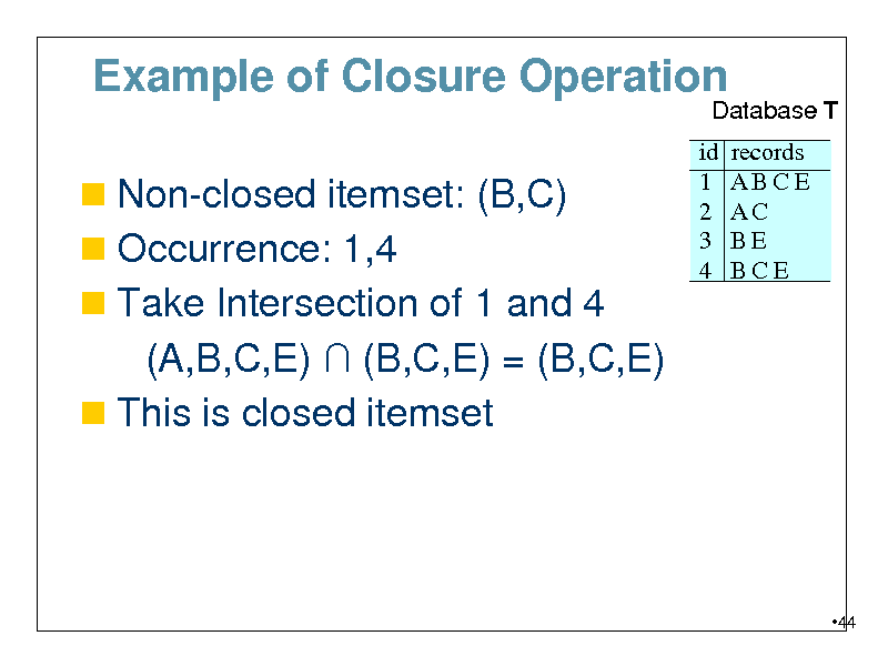
Example of Closure Operation
Database T
Non-closed itemset: (B,C) Occurrence: 1,4 Take Intersection of 1 and 4
id 1 2 3 4
records ABCE AC BE BCE
(A,B,C,E) (B,C,E) = (B,C,E) This is closed itemset
44
44
By applying the reduction map to all nodes, enumeration tree is defined.
But arrows are
in reverse direction..
{2} {7,9} {1,7,9} {2,5} {2,7,9}
{1,2,7,9}
{2,3,4,5}
{1,2,7,8,9}
{1,2,5,6,7,9} 45
45
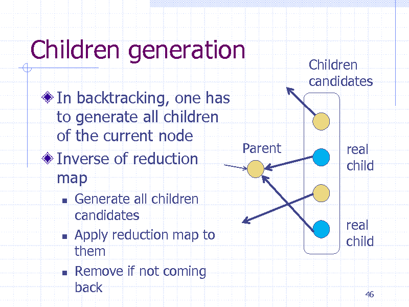
Children generation
In backtracking, one has to generate all children of the current node Parent Inverse of reduction map
Children candidates
real child
Generate all children candidates Apply reduction map to them Remove if not coming back
real child
46
46
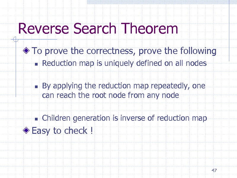
Reverse Search Theorem
To prove the correctness, prove the following
Reduction map is uniquely defined on all nodes By applying the reduction map repeatedly, one can reach the root node from any node Children generation is inverse of reduction map
Easy to check !
47
47
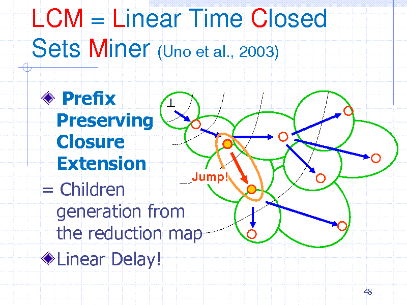
LCM = Linear Time Closed Sets Miner (Uno et al., 2003)
Prefix Preserving Closure Extension Jump! = Children generation from the reduction map Linear Delay!
48
48
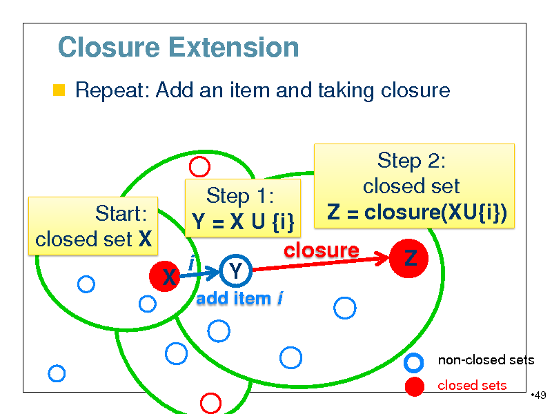
Closure Extension
Repeat: Add an item and taking closure
Step 1: Start: Y = X U {i} closed set X closure closure(X) i Y X
add item i
Step 2: closed set Z = closure(XU{i}) Z
non-closed sets closed sets
49
49
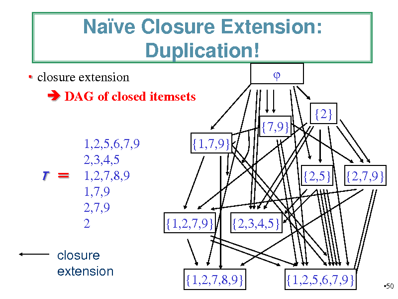
Nave Closure Extension: Duplication!
closure extension DAG of closed itemsets {2} {7,9} 1,2,5,6,7,9 2,3,4,5 1,2,7,8,9 1,7,9 2,7,9 2 {1,7,9} {2,5} {2,7,9}
T
{1,2,7,9}
{2,3,4,5}
closure extension
{1,2,7,8,9}
{1,2,5,6,7,9}
50
50
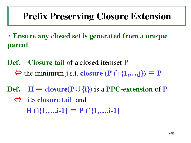
Prefix Preserving Closure Extension
Ensure any closed set is generated from a unique parent Def. Closure tail of a closed itemset P the minimum j s.t. closure (P {1,,j}) P Def. H closure(P{i}) is a PPC-extension of P i > closure tail and H {1,,i-1} P {1,,i-1}
51
51
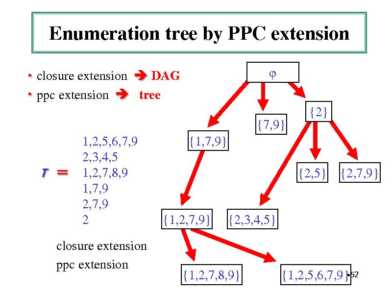
Enumeration tree by PPC extension
closure extension DAG ppc extension tree {2} {7,9} 1,2,5,6,7,9 2,3,4,5 1,2,7,8,9 1,7,9 2,7,9 2 {1,7,9} {2,5} {2,7,9}
T
{1,2,7,9}
{2,3,4,5}
closure extension ppc extension
{1,2,7,8,9}
52 {1,2,5,6,7,9}
52
![Slide: Linear Delay in Pattern Size
(Uno, Uchida, Asai, Arimura, Discovery Science 2004)
Theorem : The algorithm LCM finds all frequent closed sets X appearing in a collection of a transaction database D in O(lmn) time per closed set in the total size of D without duplicates, where l is the maximum length of transactions in D, and n is the total size of D, m is the size of pattern X.
Note: The output polynomial time complexity of Closed sets discovery is shown by [Makino et al. STACS2002]
53](https://yosinski.com/mlss12/media/slides/MLSS-2012-Tsuda-Graph-Mining_053.png)
Linear Delay in Pattern Size
(Uno, Uchida, Asai, Arimura, Discovery Science 2004)
Theorem : The algorithm LCM finds all frequent closed sets X appearing in a collection of a transaction database D in O(lmn) time per closed set in the total size of D without duplicates, where l is the maximum length of transactions in D, and n is the total size of D, m is the size of pattern X.
Note: The output polynomial time complexity of Closed sets discovery is shown by [Makino et al. STACS2002]
53
53
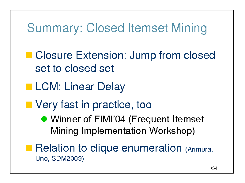
Summary: Closed Itemset Mining
Closure Extension: Jump from closed
set to closed set
LCM: Linear Delay
Very fast in practice, too
Winner of FIMI04 (Frequent Itemset Mining Implementation Workshop)
Relation to clique enumeration (Arimura,
Uno, SDM2009)
54
54
Part 4: Ordered Tree Mining
55
55
![Slide: Frequent Ordered Tree Mining
Natural extension of frequent itemset
mining problem for trees
Finding all frequent substructure in a given collection of labeled trees How to enumerate them without duplicates
Efficient DFS Algorithm
FREQT [Asai, Arimura, SIAM DM2002] TreeMiner [Zaki, ACM KDD2002] Rightmost expansion technique
56](https://yosinski.com/mlss12/media/slides/MLSS-2012-Tsuda-Graph-Mining_056.png)
Frequent Ordered Tree Mining
Natural extension of frequent itemset
mining problem for trees
Finding all frequent substructure in a given collection of labeled trees How to enumerate them without duplicates
Efficient DFS Algorithm
FREQT [Asai, Arimura, SIAM DM2002] TreeMiner [Zaki, ACM KDD2002] Rightmost expansion technique
56
56
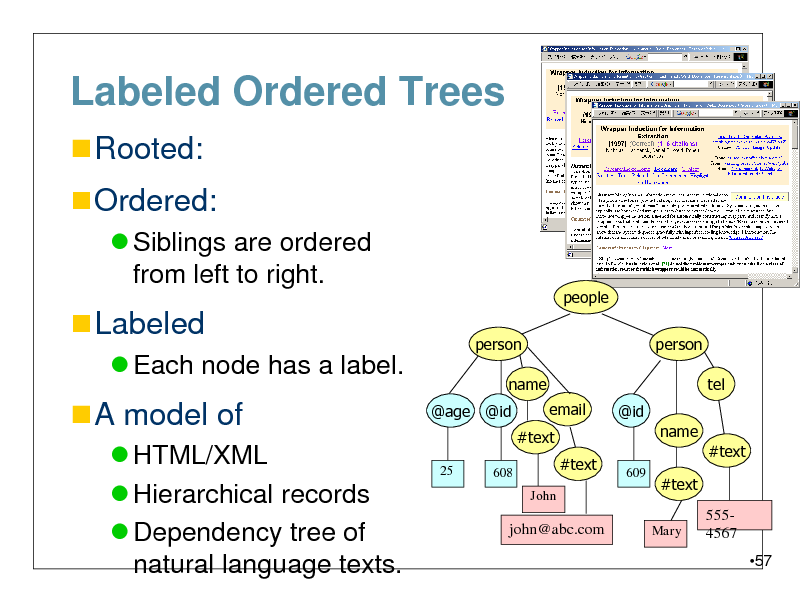
Labeled Ordered Trees
Rooted:
Ordered:
Siblings are ordered from left to right.
people person name @age @id email #text
25 608 John
Labeled
Each node has a label.
person tel @id
A model of
HTML/XML Hierarchical records Dependency tree of natural language texts.
name
#text #text
609
#text
Mary
john@abc.com
5554567 57
57
Matching between trees
Pattern tree T matches a data tree D
(T occurs in D ) pattern tree T matching function f
There is a matching function f from T into D.
A C
1
r
data tree D
B
f is 1-to-1. B f preserves parent-child relation. 3 f preserves (indirect) sibling
2 4
A A
5 6
7
C
11
C B
9
8
A
10
B
relation. f preserves labels.
B
C
58
58
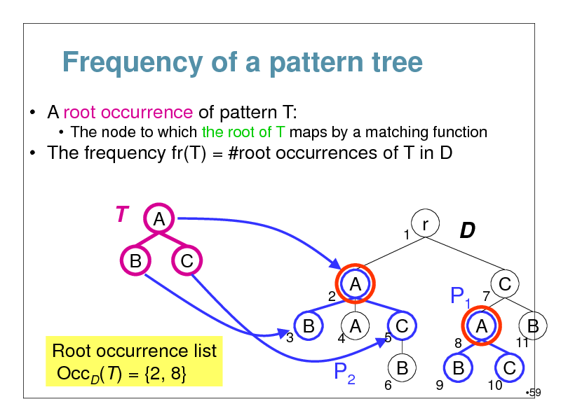
Frequency of a pattern tree
A root occurrence of pattern T:
The node to which the root of T maps by a matching function
The frequency fr(T) = #root occurrences of T in D
T
B
A
1
r
D
P1
7
C
2 3
A
4
C B
11
B
A
Root occurrence list OccD(T) = {2, 8}
5 6
C
8
A B
9 10
P2
B
C
59
59
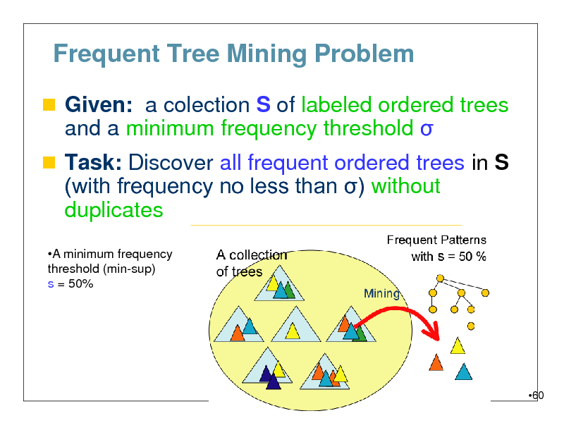
Frequent Tree Mining Problem
Given: a colection S of labeled ordered trees
and a minimum frequency threshold
Task: Discover all frequent ordered trees in S (with frequency no less than ) without
duplicates
A minimum frequency threshold (min-sup) s = 50%
60
60
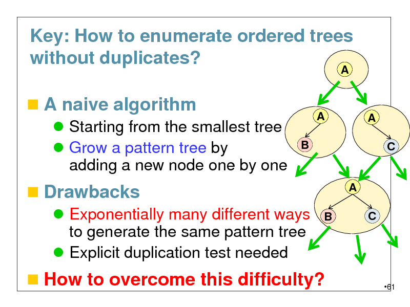
Key: How to enumerate ordered trees without duplicates?
A
A naive algorithm
Starting from the smallest tree Grow a pattern tree by adding a new node one by one
B
A
A C
Drawbacks
Exponentially many different ways to generate the same pattern tree Explicit duplication test needed
B
A C
How to overcome this difficulty?
61
61
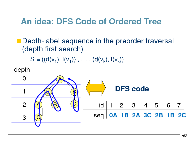
An idea: DFS Code of Ordered Tree
Depth-label sequence in the preorder traversal
(depth first search)
S = ((d(v1), l(v1)) , , (d(vk), l(vk)) depth 0 1
B
A C B A
B C
DFS code
id 1 2 3 4 5 6 7
2
3
seq 0A 1B 2A 3C 2B 1B 2C
62
62
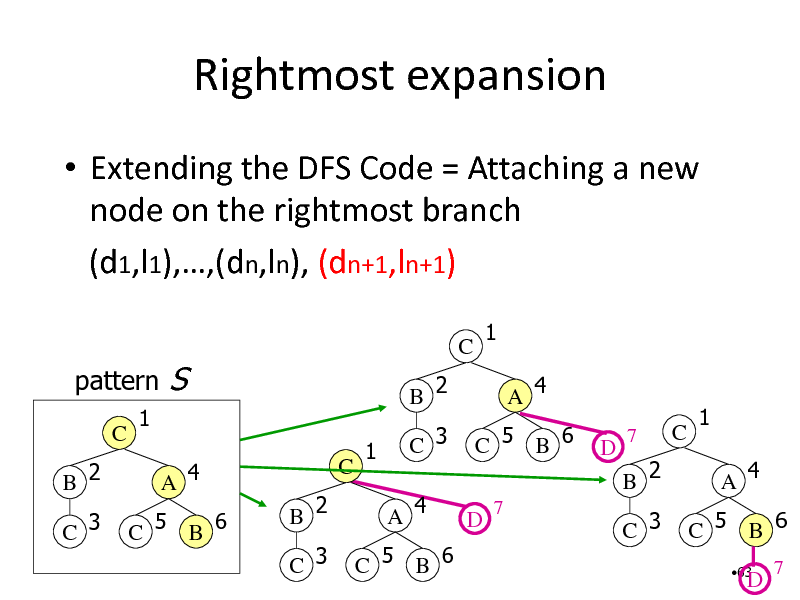
Rightmost expansion
Extending the DFS Code = Attaching a new node on the rightmost branch (d1,l1),,(dn,ln), (dn+1,ln+1)
pattern
C B 2 C 3 1 A 4 C 5 B 6
S
C
B 2 C 3
C B 2
1 A 4
1
C 3
A 4
C 5 B 6
D
7
D
7
C
1 A 4 C 5 B 6
63
B 2 C 3
C 5 B 6
D
7
63
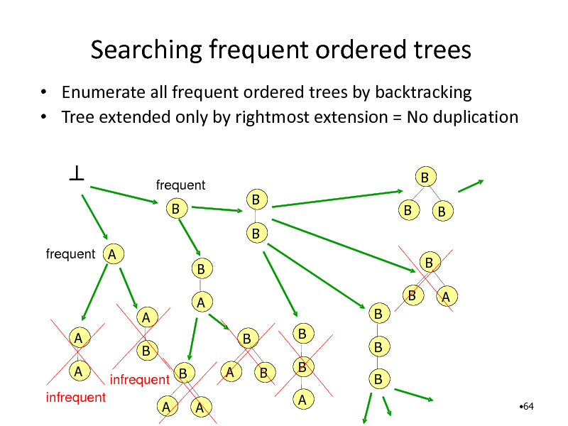
Searching frequent ordered trees
Enumerate all frequent ordered trees by backtracking Tree extended only by rightmost extension = No duplication
frequent B
B B B B B
frequent A
B A
B B B B A B B B A B A
A
A
A infrequent
B infrequent B A A
B
64
64
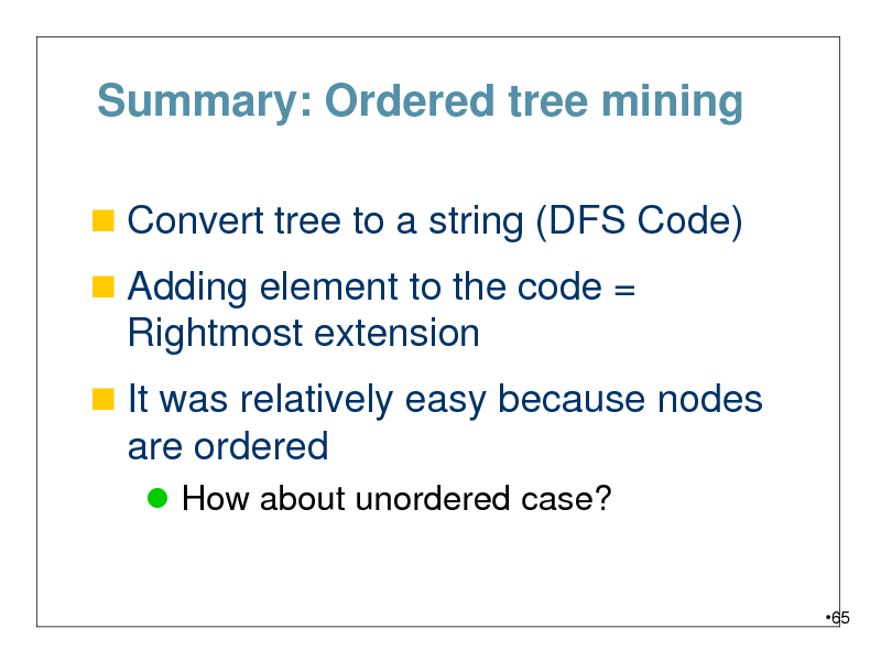
Summary: Ordered tree mining
Convert tree to a string (DFS Code)
Adding element to the code =
Rightmost extension
It was relatively easy because nodes
are ordered
How about unordered case?
65
65
Part 5: Unordered Tree Mining
66
66
![Slide: Frequent Unordered Tree Mining
Unordered trees: Non-trivial subclass of general graphs Problem: Exponentially many isomorphic trees Efficient DFS Algorithm
A
B B
A B A C
B
A
B
C
B
C
Unot [Asai, Arimura, DS'03] NK [Nijssen, Kok, MGTS03]
C
A B C B
A
B B
C B
B
A
A
C
C
67](https://yosinski.com/mlss12/media/slides/MLSS-2012-Tsuda-Graph-Mining_067.png)
Frequent Unordered Tree Mining
Unordered trees: Non-trivial subclass of general graphs Problem: Exponentially many isomorphic trees Efficient DFS Algorithm
A
B B
A B A C
B
A
B
C
B
C
Unot [Asai, Arimura, DS'03] NK [Nijssen, Kok, MGTS03]
C
A B C B
A
B B
C B
B
A
A
C
C
67
67
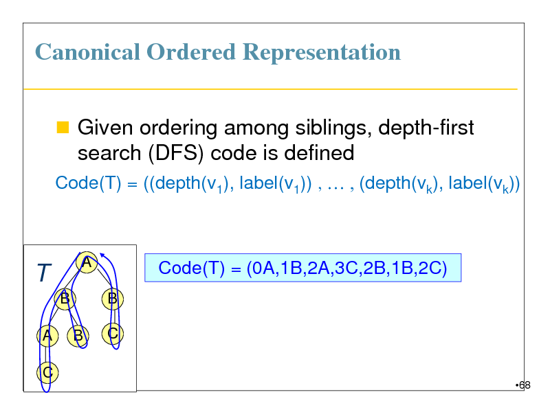
Canonical Ordered Representation
Given ordering among siblings, depth-first search (DFS) code is defined
Code(T) = ((depth(v1), label(v1)) , , (depth(vk), label(vk))
T
B
A C
A
Code(T) = (0A,1B,2A,3C,2B,1B,2C)
B
B
C
68
68
Canonical representation
Ordered tree T with lexicographically maximum code
T1
B A
C
(0A,1B,2A,3C,2B,1B,2C)
A
T2
B C
A
T3
B B C C
A
T4
B B B C
A
B
B B A
C
B
B
A
C
A
C
(0A,1B,2B,2A,3C,1B,2C)
(0A,1B,2C,1B,2A,3C,2B)
(0A,1B,2C,1B,2B,2A,3C) 69
69
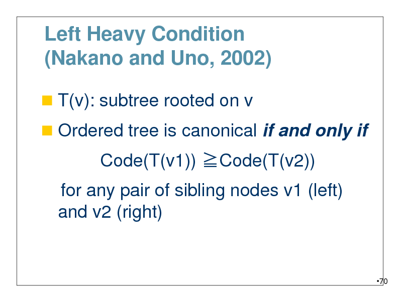
Left Heavy Condition (Nakano and Uno, 2002)
T(v): subtree rooted on v
Ordered tree is canonical if and only if
Code(T(v1)) Code(T(v2))
for any pair of sibling nodes v1 (left) and v2 (right)
70
70
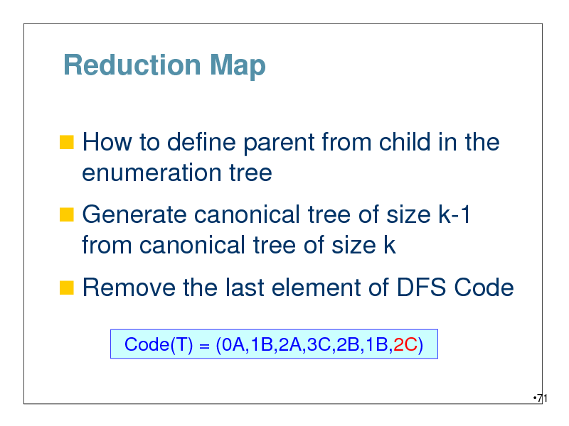
Reduction Map
How to define parent from child in the
enumeration tree
Generate canonical tree of size k-1
from canonical tree of size k
Remove the last element of DFS Code
Code(T) = (0A,1B,2A,3C,2B,1B,2C)
71
71
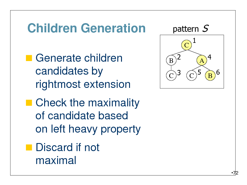
Children Generation
Generate children
pattern
C B 2 C 3 1
S
A 4
candidates by rightmost extension
Check the maximality
C 5 B 6
of candidate based on left heavy property
Discard if not
maximal
72
72
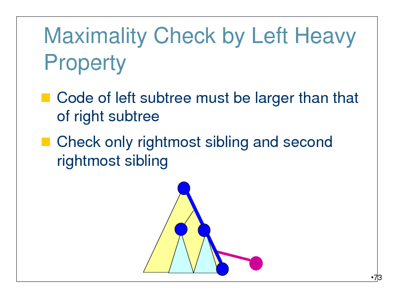
Maximality Check by Left Heavy Property
Code of left subtree must be larger than that of right subtree
Check only rightmost sibling and second rightmost sibling
73
73
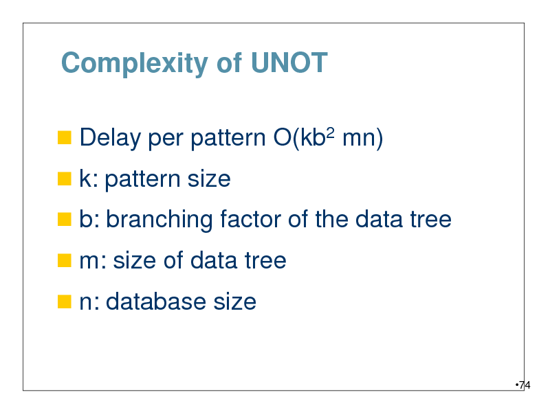
Complexity of UNOT
Delay per pattern O(kb2 mn)
k: pattern size
b: branching factor of the data tree
m: size of data tree
n: database size
74
74
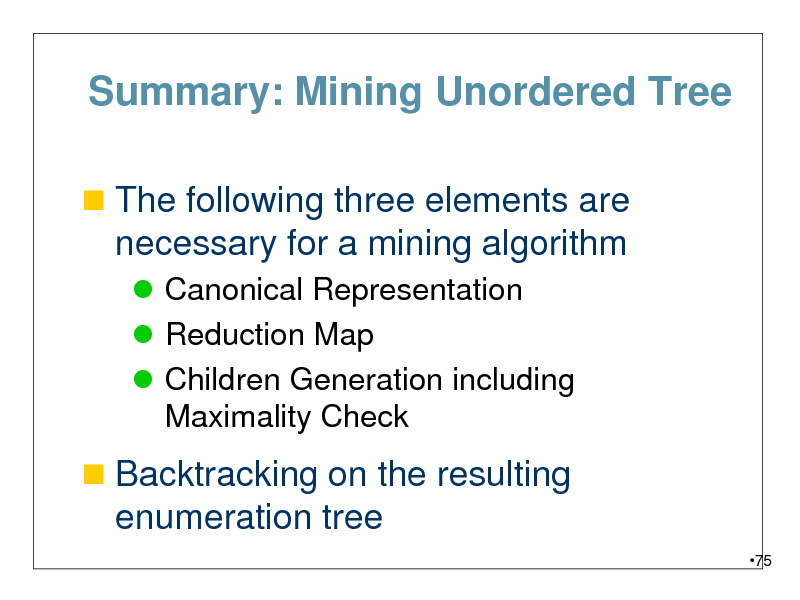
Summary: Mining Unordered Tree
The following three elements are
necessary for a mining algorithm
Canonical Representation Reduction Map Children Generation including Maximality Check
Backtracking on the resulting
enumeration tree
75
75
Part 6: Graph Mining
76
76
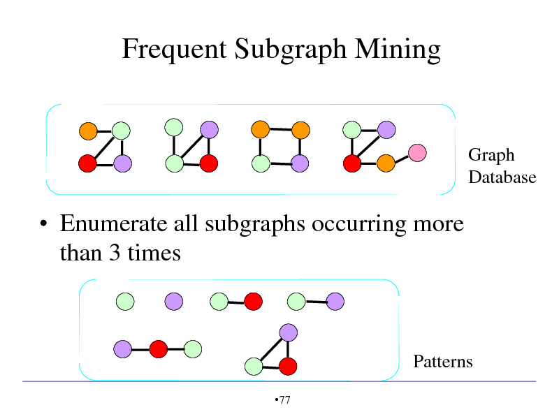
Frequent Subgraph Mining
Graph Database
Enumerate all subgraphs occurring more than 3 times
Patterns
77
77
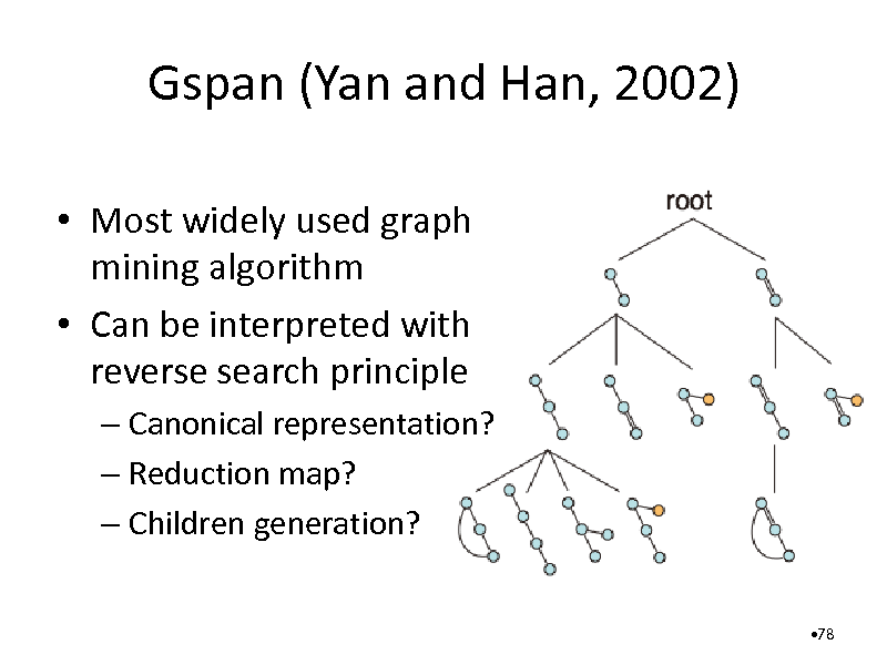
Gspan (Yan and Han, 2002)
Most widely used graph mining algorithm Can be interpreted with reverse search principle
Canonical representation? Reduction map? Children generation?
78
78
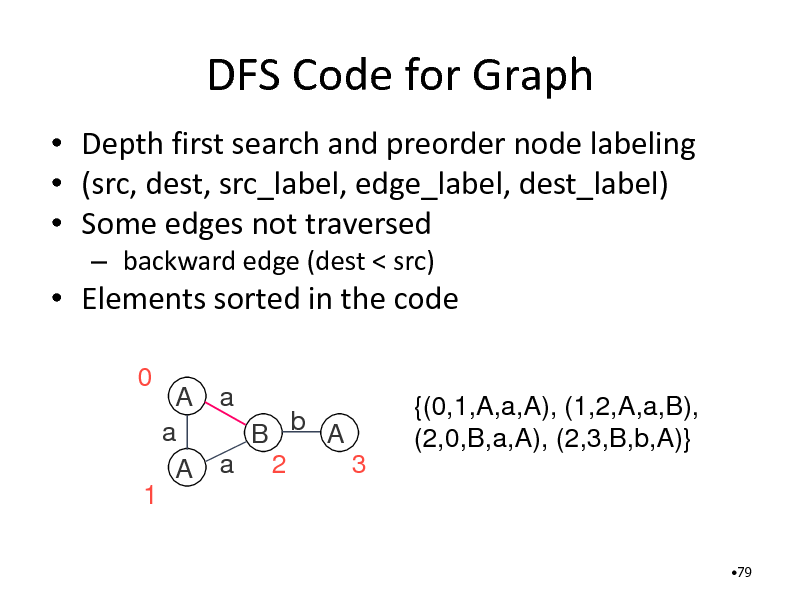
DFS Code for Graph
Depth first search and preorder node labeling (src, dest, src_label, edge_label, dest_label) Some edges not traversed
backward edge (dest < src)
Elements sorted in the code
0 A a a B b A 3 A a 2 {(0,1,A,a,A), (1,2,A,a,B), (2,0,B,a,A), (2,3,B,b,A)}
1
79
79
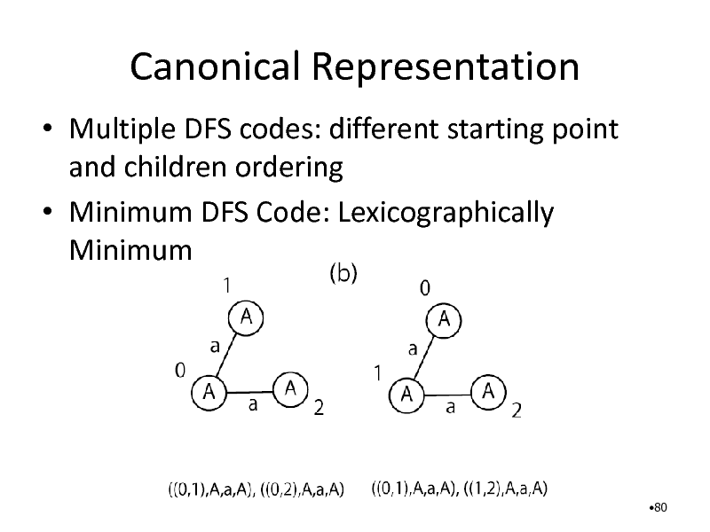
Canonical Representation
Multiple DFS codes: different starting point and children ordering Minimum DFS Code: Lexicographically Minimum
80
80
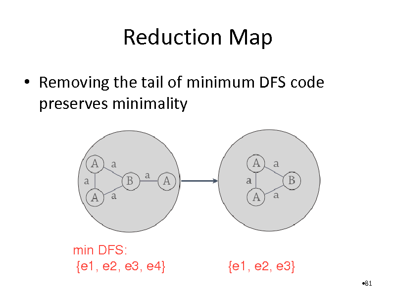
Reduction Map
Removing the tail of minimum DFS code preserves minimality
min DFS: {e1, e2, e3, e4}
{e1, e2, e3}
81
81
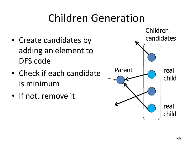
Children Generation
Create candidates by adding an element to DFS code Check if each candidate is minimum If not, remove it
Children candidates
Parent
real child
real child
82
82
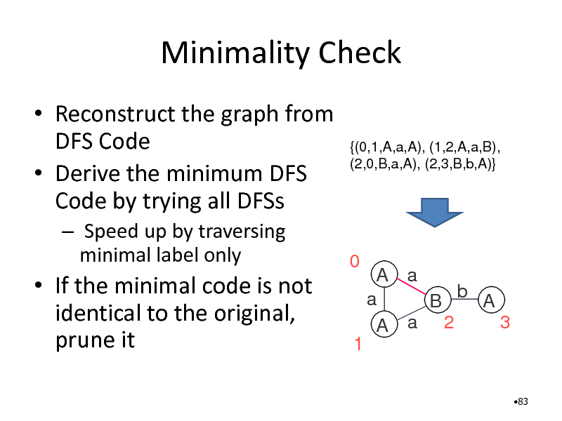
Minimality Check
Reconstruct the graph from DFS Code Derive the minimum DFS Code by trying all DFSs
Speed up by traversing minimal label only
{(0,1,A,a,A), (1,2,A,a,B), (2,0,B,a,A), (2,3,B,b,A)}
If the minimal code is not identical to the original, prune it
0
A a a B b A 3 A a 2
1
83
83
Summary: Graph Mining
gSpan is a typical example of reverse search Not explained: Closed tree mining, Closed Graph mining Delay exponential to pattern size
It cannot be avoided due to NP-hardness of graph isomorphism Yet it scales to millions for sparse molecular graphs
Applications covered in next chapter
84
84
Part7: Dense Module Enumeration
85
85
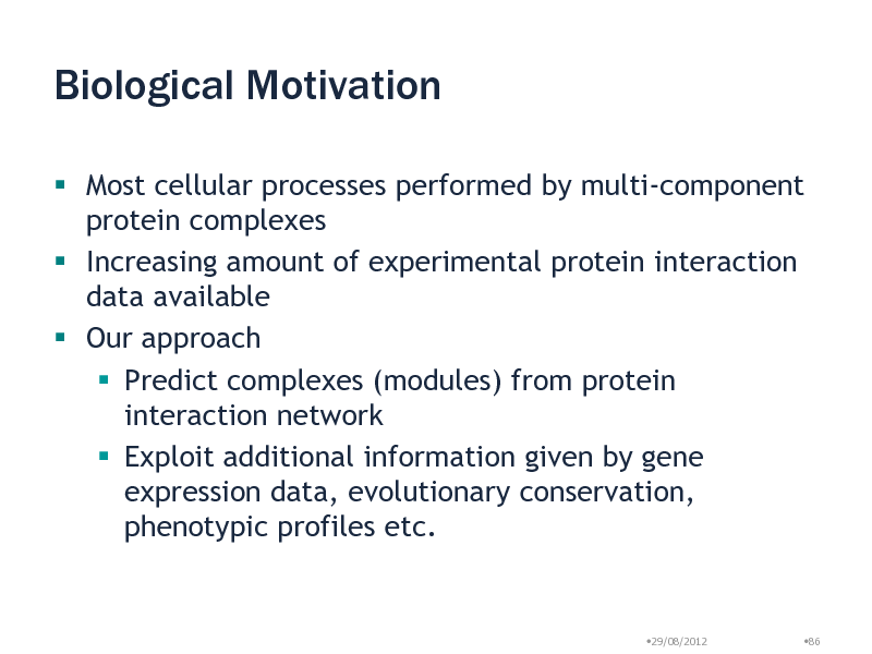
Biological Motivation
Most cellular processes performed by multi-component protein complexes Increasing amount of experimental protein interaction data available Our approach Predict complexes (modules) from protein interaction network Exploit additional information given by gene expression data, evolutionary conservation, phenotypic profiles etc.
29/08/2012
86
86
29/08/2012
87
87
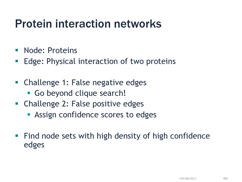
Protein interaction networks
Node: Proteins Edge: Physical interaction of two proteins
Challenge 1: False negative edges Go beyond clique search! Challenge 2: False positive edges Assign confidence scores to edges Find node sets with high density of high confidence edges
29/08/2012
88
88
![Slide: Module Discovery
Previous work Clique percolation [Palla et al., 2005] Partitioning
Hierarchical clustering [Girvan and Newman, 2001] Flow Simulation [Krogan et al., 2006] Spectral methods [Newman, 2006]
Heuristic Local Search [Bader and Hogue, 2003]
Our approach Exhaustively enumerate all dense subgraphs efficiently
29/08/2012
89](https://yosinski.com/mlss12/media/slides/MLSS-2012-Tsuda-Graph-Mining_089.png)
Module Discovery
Previous work Clique percolation [Palla et al., 2005] Partitioning
Hierarchical clustering [Girvan and Newman, 2001] Flow Simulation [Krogan et al., 2006] Spectral methods [Newman, 2006]
Heuristic Local Search [Bader and Hogue, 2003]
Our approach Exhaustively enumerate all dense subgraphs efficiently
29/08/2012
89
89
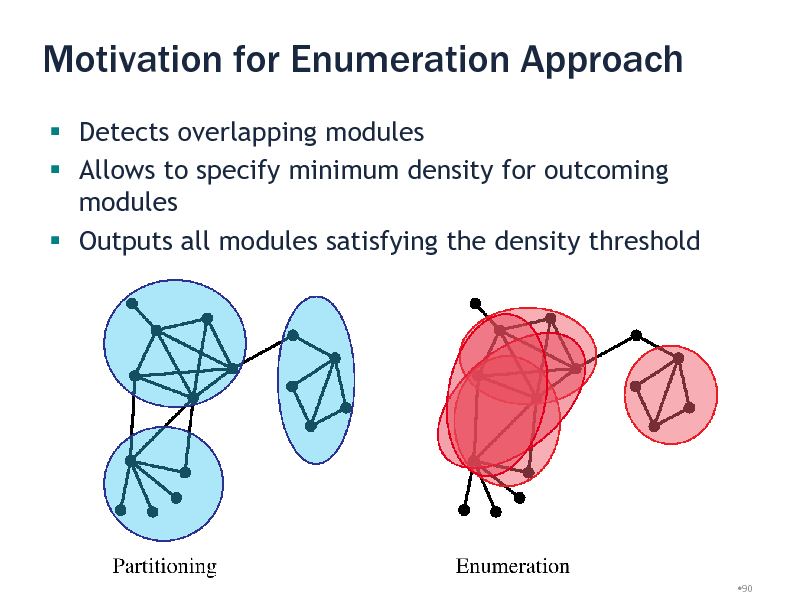
Motivation for Enumeration Approach
Detects overlapping modules Allows to specify minimum density for outcoming modules Outputs all modules satisfying the density threshold
29/08/2012
90
90
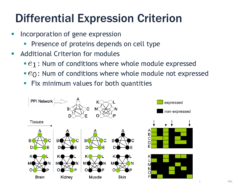
Differential Expression Criterion
Incorporation of gene expression Presence of proteins depends on cell type Additional Criterion for modules : Num of conditions where whole module expressed : Num of conditions where whole module not expressed Fix minimum values for both quantities
29/08/2012
91
91
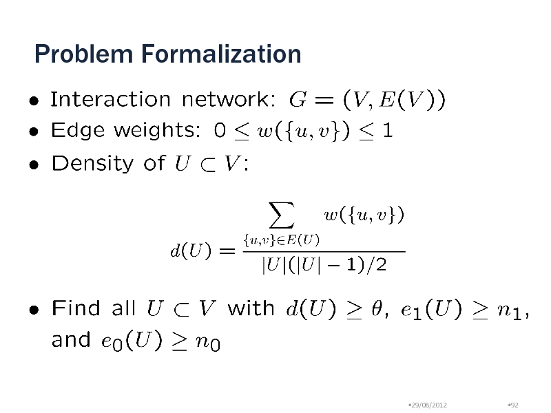
Problem Formalization
29/08/2012
92
92
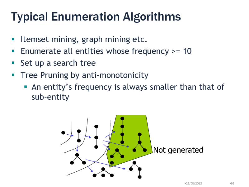
Typical Enumeration Algorithms
Itemset mining, graph mining etc. Enumerate all entities whose frequency >= 10 Set up a search tree Tree Pruning by anti-monotonicity An entitys frequency is always smaller than that of sub-entity
Not generated
29/08/2012
93
93
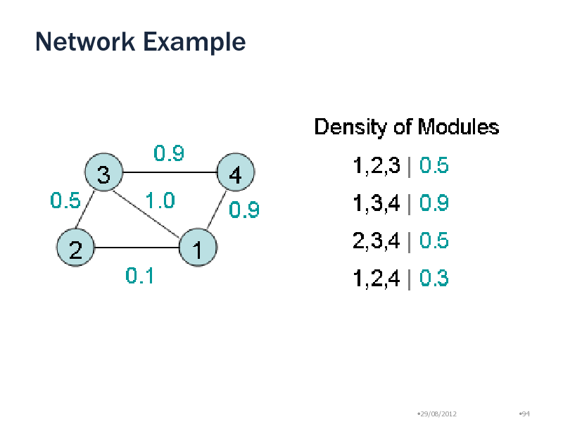
Network Example
29/08/2012
94
94
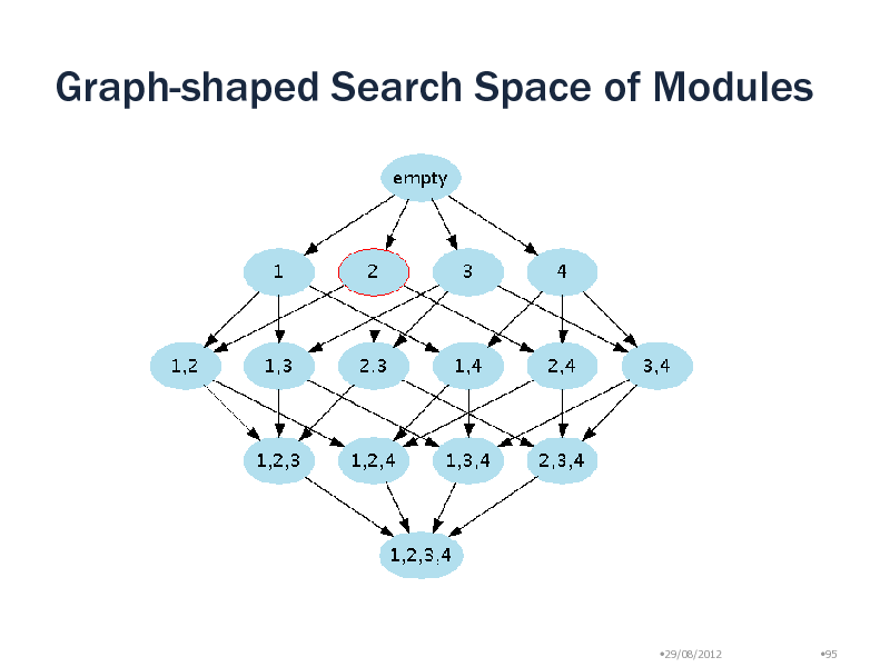
Graph-shaped Search Space of Modules
29/08/2012
95
95
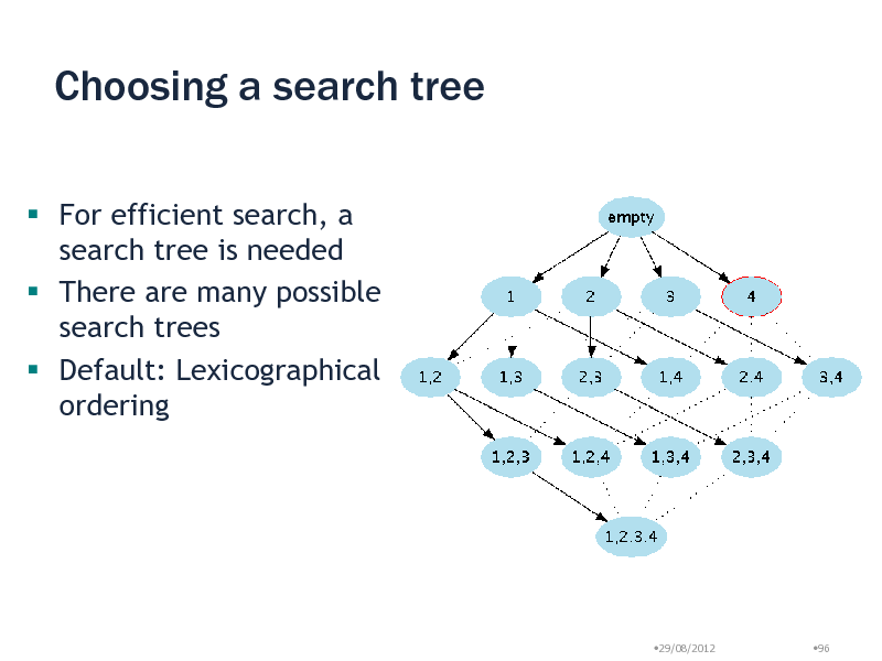
Choosing a search tree
For efficient search, a search tree is needed There are many possible search trees Default: Lexicographical ordering
29/08/2012
96
96
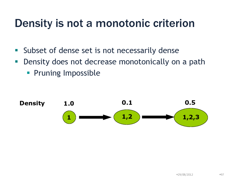
Density is not a monotonic criterion
Subset of dense set is not necessarily dense Density does not decrease monotonically on a path Pruning Impossible
Density
1.0 1
0.1 1,2
0.5 1,2,3
29/08/2012
97
97
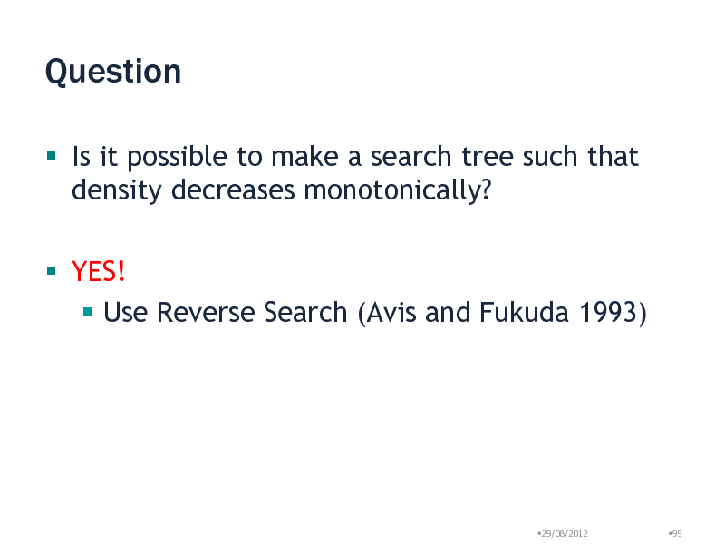
Question
Is it possible to make a search tree such that density decreases monotonically?
29/08/2012
98
98
Question
Is it possible to make a search tree such that density decreases monotonically? YES! Use Reverse Search (Avis and Fukuda 1993)
29/08/2012
99
99
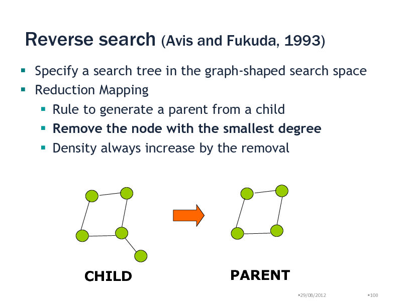
Reverse search (Avis and Fukuda, 1993)
Specify a search tree in the graph-shaped search space Reduction Mapping Rule to generate a parent from a child Remove the node with the smallest degree Density always increase by the removal
CHILD
PARENT
29/08/2012 100
100
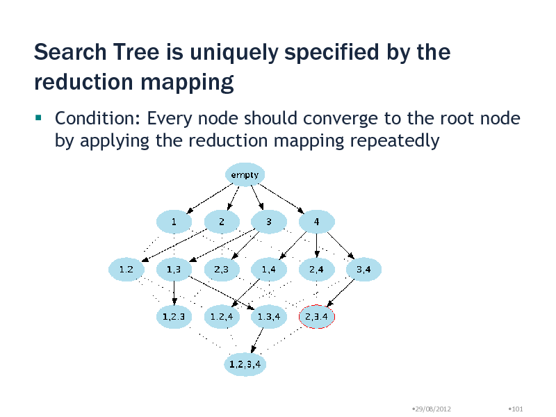
Search Tree is uniquely specified by the reduction mapping
Condition: Every node should converge to the root node by applying the reduction mapping repeatedly
29/08/2012
101
101
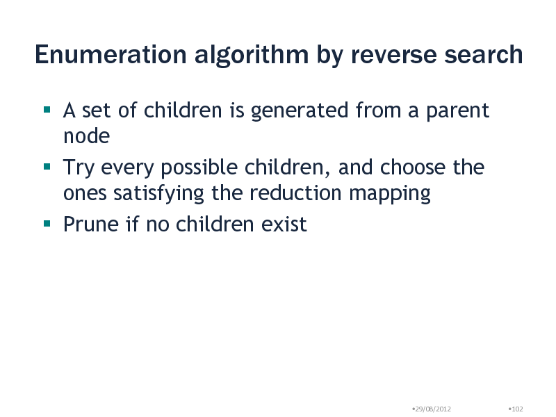
Enumeration algorithm by reverse search
A set of children is generated from a parent node Try every possible children, and choose the ones satisfying the reduction mapping Prune if no children exist
29/08/2012
102
102
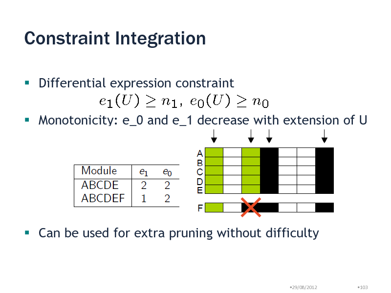
Constraint Integration
Differential expression constraint
Monotonicity: e_0 and e_1 decrease with extension of U
Can be used for extra pruning without difficulty
29/08/2012
103
103
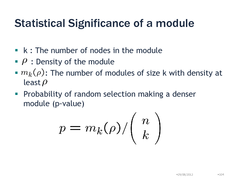
Statistical Significance of a module
k : The number of nodes in the module : Density of the module : The number of modules of size k with density at least Probability of random selection making a denser module (p-value)
29/08/2012
104
104
Benchmarking in yeast complex discovery
Combined interactions from CYGD-Mpact and DIP Interactions among 3559 nodes Confidence weights on edges due to (Jansen, 2003) Methods in comparison Clique detection (Clique) Clique Parcolation Method (CPM) Markov Clustering Modules compared with MIPS complexes
29/08/2012
105
105
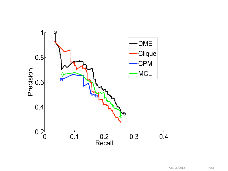
29/08/2012
106
106
Evolutionary Conserved Yeast Modules
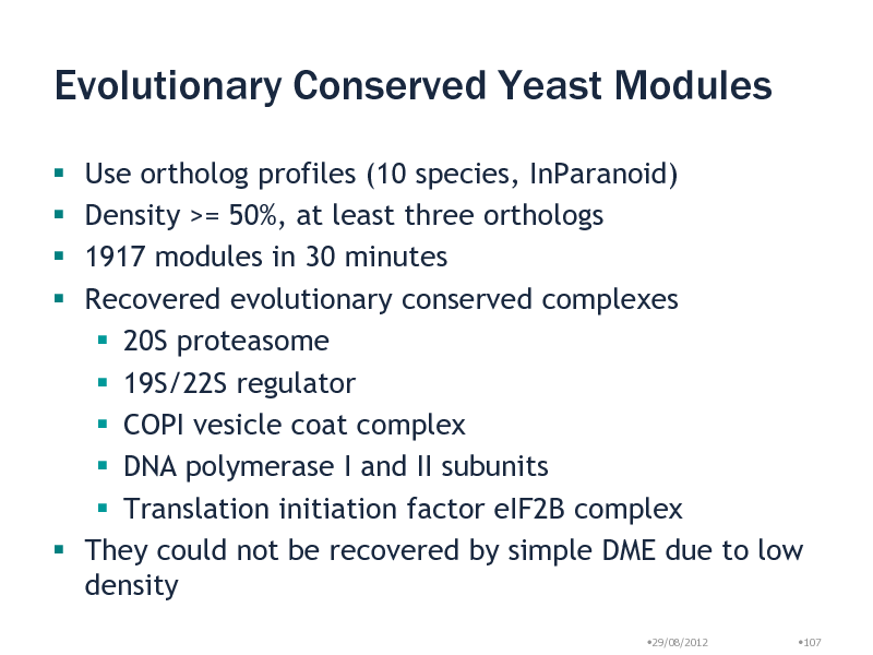
Use ortholog profiles (10 species, InParanoid) Density >= 50%, at least three orthologs 1917 modules in 30 minutes Recovered evolutionary conserved complexes 20S proteasome 19S/22S regulator COPI vesicle coat complex DNA polymerase I and II subunits Translation initiation factor eIF2B complex They could not be recovered by simple DME due to low density
29/08/2012 107
107
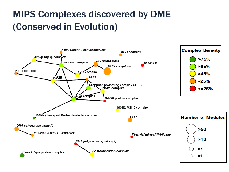
MIPS Complexes discovered by DME (Conserved in Evolution)
29/08/2012
108
108
Phenotype-associated yeast modules
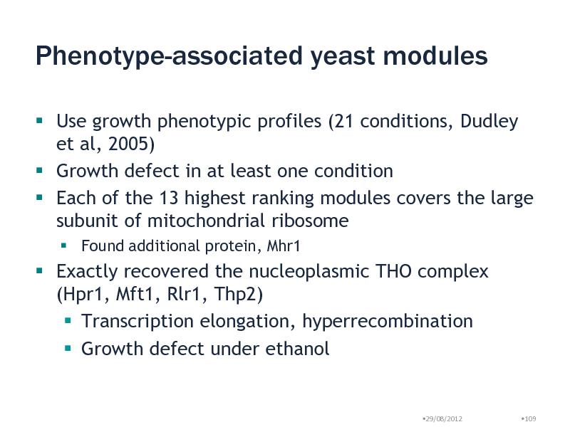
Use growth phenotypic profiles (21 conditions, Dudley et al, 2005) Growth defect in at least one condition Each of the 13 highest ranking modules covers the large subunit of mitochondrial ribosome
Found additional protein, Mhr1
Exactly recovered the nucleoplasmic THO complex (Hpr1, Mft1, Rlr1, Thp2) Transcription elongation, hyperrecombination Growth defect under ethanol
29/08/2012
109
109
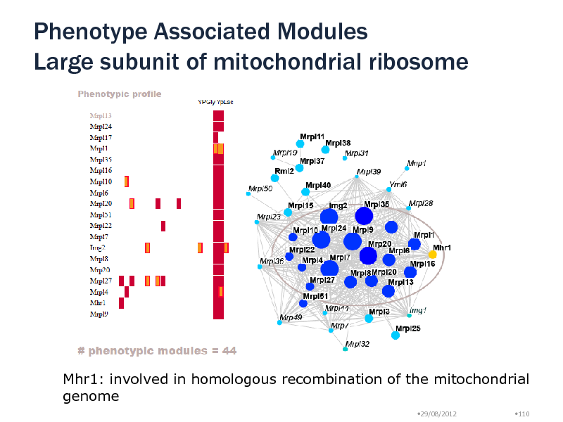
Phenotype Associated Modules Large subunit of mitochondrial ribosome
Mhr1: involved in homologous recombination of the mitochondrial genome
29/08/2012 110
110
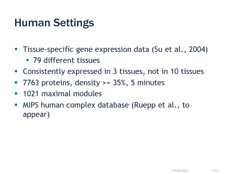
Human Settings
Tissue-specific gene expression data (Su et al., 2004) 79 different tissues Consistently expressed in 3 tissues, not in 10 tissues 7763 proteins, density >= 35%, 5 minutes 1021 maximal modules MIPS human complex database (Ruepp et al., to appear)
29/08/2012
111
111
Human-expression result
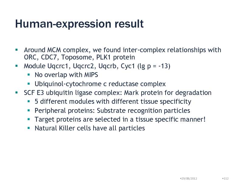
Around MCM complex, we found inter-complex relationships with ORC, CDC7, Toposome, PLK1 protein Module Uqcrc1, Uqcrc2, Uqcrb, Cyc1 (lg p = -13) No overlap with MIPS Ubiquinol-cytochrome c reductase complex SCF E3 ubiquitin ligase complex: Mark protein for degradation 5 different modules with different tissue specificity Peripheral proteins: Substrate recognition particles Target proteins are selected in a tissue specific manner! Natural Killer cells have all particles
29/08/2012
112
112
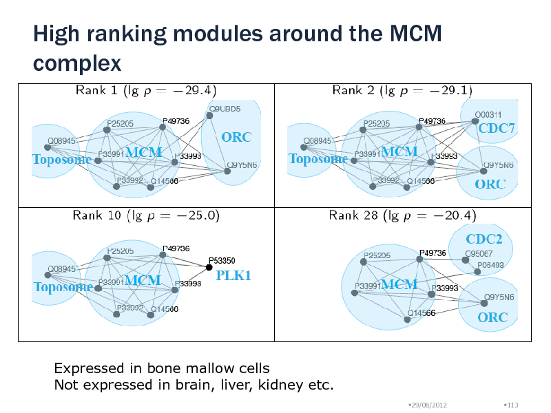
High ranking modules around the MCM complex
Expressed in bone mallow cells Not expressed in brain, liver, kidney etc.
29/08/2012 113
113
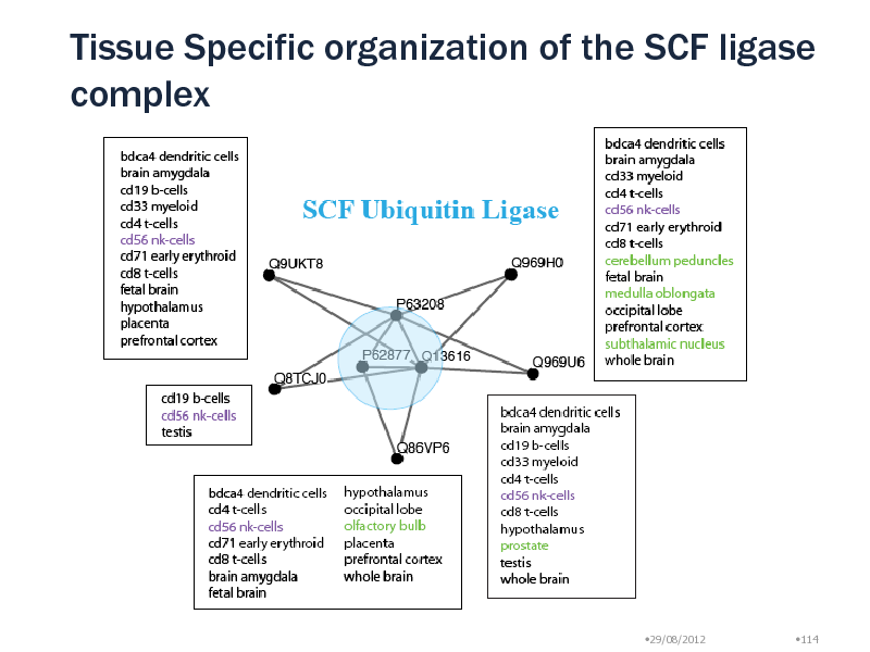
Tissue Specific organization of the SCF ligase complex
29/08/2012
114
114
Summary: Dense Module Enumeration
Novel module enumeration algorithm based on reverse search Combination with other information sources Statistical significance of dense modules Successfully applied to yeast/human protein interaction networks
29/08/2012
115
115
![Slide: Reference
[1] R. Agrawal and R. Srikant, Fast algorithms for mining association rules, in Proc. 20th Int. Conf. Very Large Data Bases, 1994. [2] T. Asai, H. Arimura, T. Uno, and S. Nakano, Discovering frequent substructures in large unordered trees, Discovery science, 2003. [3] T. Asai, K. Abe, S. Kawasoe, H. Arimura, H. Sakamoto, and S. Arikawa, Efficient Substructure Discovery from Large Semi-structured Data., in SDM, 2002. [4] D. Avis and K. Fukuda, Reverse search for enumeration, Discrete Applied Mathematics, vol. 65, no. 13, pp. 2146, 1996. [5] E. Georgii, S. Dietmann, T. Uno, P. Pagel, and K. Tsuda, Enumeration of conditiondependent dense modules in protein interaction networks., Bioinformatics (Oxford, England), vol. 25, no. 7, pp. 93340, Apr. 2009. [6] S. Nijssen and J. Kok, Efficient discovery of frequent unordered trees, MGTS, 2003. [7] N. Pasquier, Y. Bastide, R. Taouil, and L. Lakhal, Discovering frequent closed itemsets for association rules, Database TheoryICDT99, 1999. [8] I. Takigawa and H. Mamitsuka, Efficiently mining -tolerance closed frequent subgraphs, Machine Learning, vol. 82, no. 2, pp. 95121, Sep. 2010. [9] X. Yan and J. Han, gSpan: graph-based substructure pattern mining, in 2002 IEEE International Conference on Data Mining, 2002. Proceedings., pp. 721724. [10] M. Zaki, Efficiently mining frequent trees in a forest: Algorithms and applications, IEEE Transaction on Knowledge and Data Engineering, 2005.
29/08/2012 116](https://yosinski.com/mlss12/media/slides/MLSS-2012-Tsuda-Graph-Mining_116.png)
Reference
[1] R. Agrawal and R. Srikant, Fast algorithms for mining association rules, in Proc. 20th Int. Conf. Very Large Data Bases, 1994. [2] T. Asai, H. Arimura, T. Uno, and S. Nakano, Discovering frequent substructures in large unordered trees, Discovery science, 2003. [3] T. Asai, K. Abe, S. Kawasoe, H. Arimura, H. Sakamoto, and S. Arikawa, Efficient Substructure Discovery from Large Semi-structured Data., in SDM, 2002. [4] D. Avis and K. Fukuda, Reverse search for enumeration, Discrete Applied Mathematics, vol. 65, no. 13, pp. 2146, 1996. [5] E. Georgii, S. Dietmann, T. Uno, P. Pagel, and K. Tsuda, Enumeration of conditiondependent dense modules in protein interaction networks., Bioinformatics (Oxford, England), vol. 25, no. 7, pp. 93340, Apr. 2009. [6] S. Nijssen and J. Kok, Efficient discovery of frequent unordered trees, MGTS, 2003. [7] N. Pasquier, Y. Bastide, R. Taouil, and L. Lakhal, Discovering frequent closed itemsets for association rules, Database TheoryICDT99, 1999. [8] I. Takigawa and H. Mamitsuka, Efficiently mining -tolerance closed frequent subgraphs, Machine Learning, vol. 82, no. 2, pp. 95121, Sep. 2010. [9] X. Yan and J. Han, gSpan: graph-based substructure pattern mining, in 2002 IEEE International Conference on Data Mining, 2002. Proceedings., pp. 721724. [10] M. Zaki, Efficiently mining frequent trees in a forest: Algorithms and applications, IEEE Transaction on Knowledge and Data Engineering, 2005.
29/08/2012 116
116
Machine Learning Summer School Kyoto 2012
Graph Mining
Chapter 2: Learning from Structured Data
National Institute of Advanced Industrial Science and Technology Koji Tsuda
1
117
Agenda 2 (Learning from Structured Data)
1. 2. 3. 4. 5. Preliminaries Graph Clustering by EM Graph Boosting Regularization Paths in Graph Classification Itemset Boosting for predicting HIV drug resistance
2
118

Part 1: Preliminaries
3
119
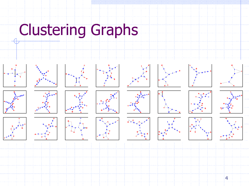
Clustering Graphs
4
120
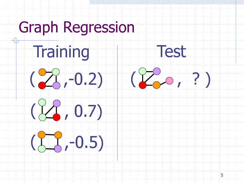
Graph Regression
Training ( (
( ,-0.2) , 0.7) ,-0.5) (
Test
, ?)
5
121
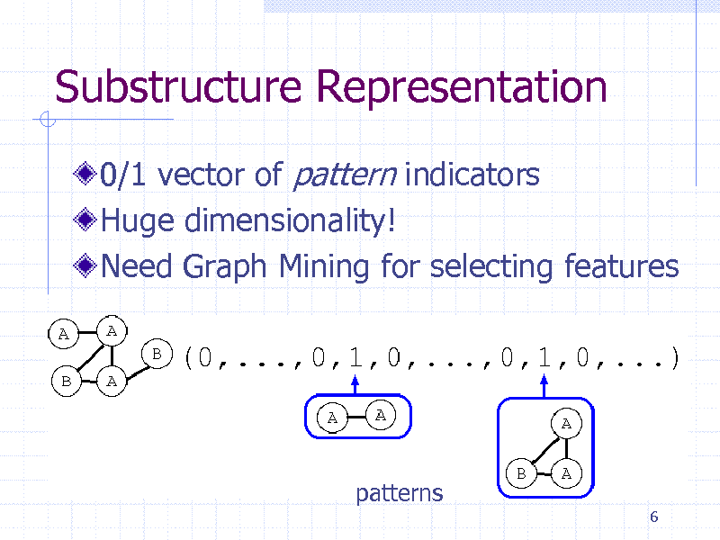
Substructure Representation
0/1 vector of pattern indicators Huge dimensionality! Need Graph Mining for selecting features
patterns
6
122
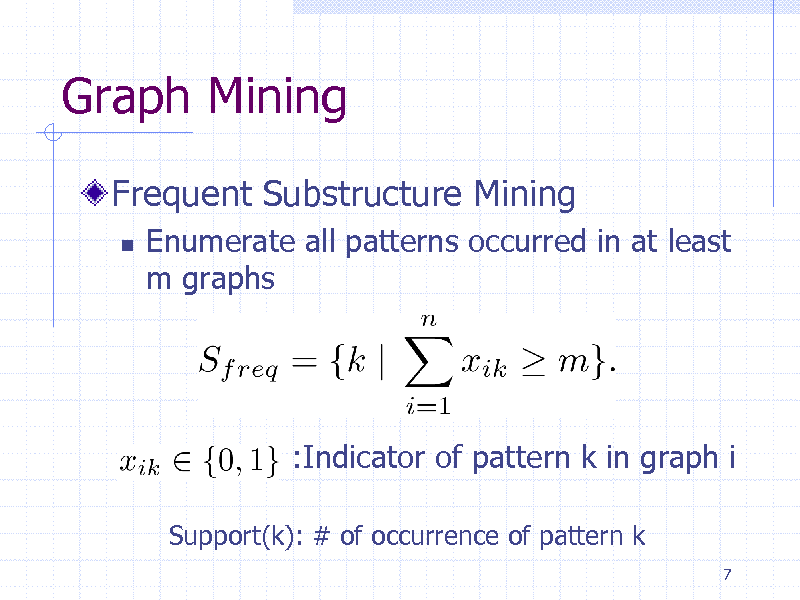
Graph Mining
Frequent Substructure Mining
Enumerate all patterns occurred in at least m graphs
:Indicator of pattern k in graph i
Support(k): # of occurrence of pattern k
7
123
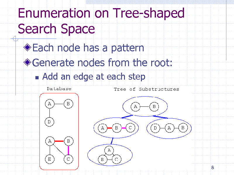
Enumeration on Tree-shaped Search Space
Each node has a pattern Generate nodes from the root:
Add an edge at each step
8
124
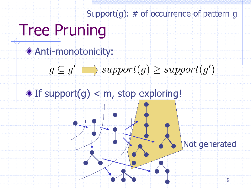
Support(g): # of occurrence of pattern g
Tree Pruning
Anti-monotonicity:
If support(g) < m, stop exploring!
Not generated
9
125
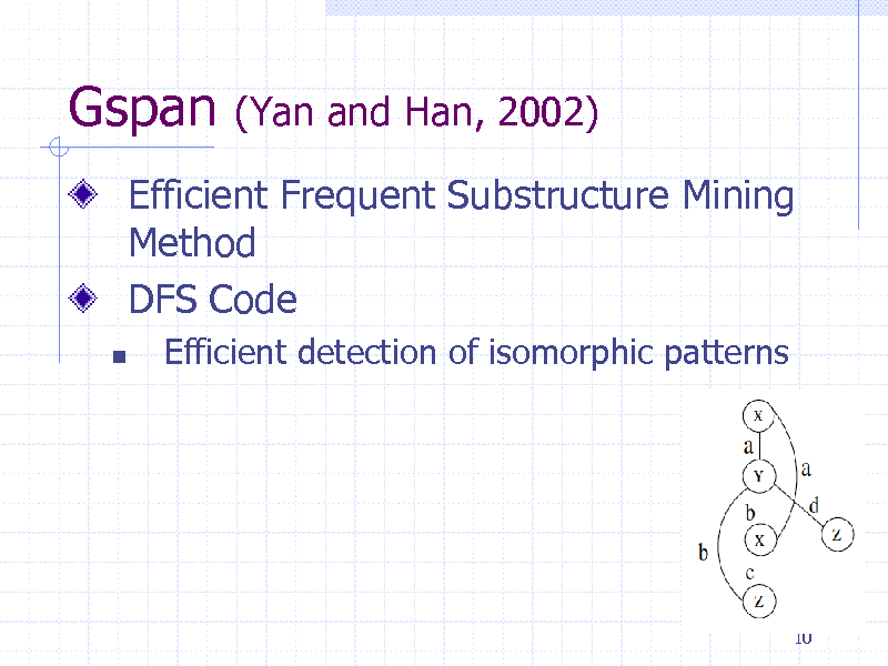
Gspan
(Yan and Han, 2002)
Efficient Frequent Substructure Mining Method DFS Code
Efficient detection of isomorphic patterns
10
126
![Slide: Depth First Search (DFS) Code
A labeled graph G A a B 1 c b b A 2 [1,2,B,c,A] [0,3,A,b,C] [0,1,A,a,B] [0,2,A,b,A]
G0
0
C
3
DFS Code Tree on G
[2,0,A,b,A] [0,3,A,b,C]
Isomorphic
[0,1,A,a,B]
G1
[2,0,A,b,A] [0,3,A,b,C]
[0,3,A,b,C]
Non-minimum DFS code. Prune it. 11](https://yosinski.com/mlss12/media/slides/MLSS-2012-Tsuda-Graph-Mining_127.png)
Depth First Search (DFS) Code
A labeled graph G A a B 1 c b b A 2 [1,2,B,c,A] [0,3,A,b,C] [0,1,A,a,B] [0,2,A,b,A]
G0
0
C
3
DFS Code Tree on G
[2,0,A,b,A] [0,3,A,b,C]
Isomorphic
[0,1,A,a,B]
G1
[2,0,A,b,A] [0,3,A,b,C]
[0,3,A,b,C]
Non-minimum DFS code. Prune it. 11
127
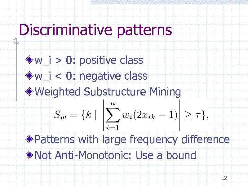
Discriminative patterns
w_i > 0: positive class w_i < 0: negative class Weighted Substructure Mining
Patterns with large frequency difference Not Anti-Monotonic: Use a bound
12
128
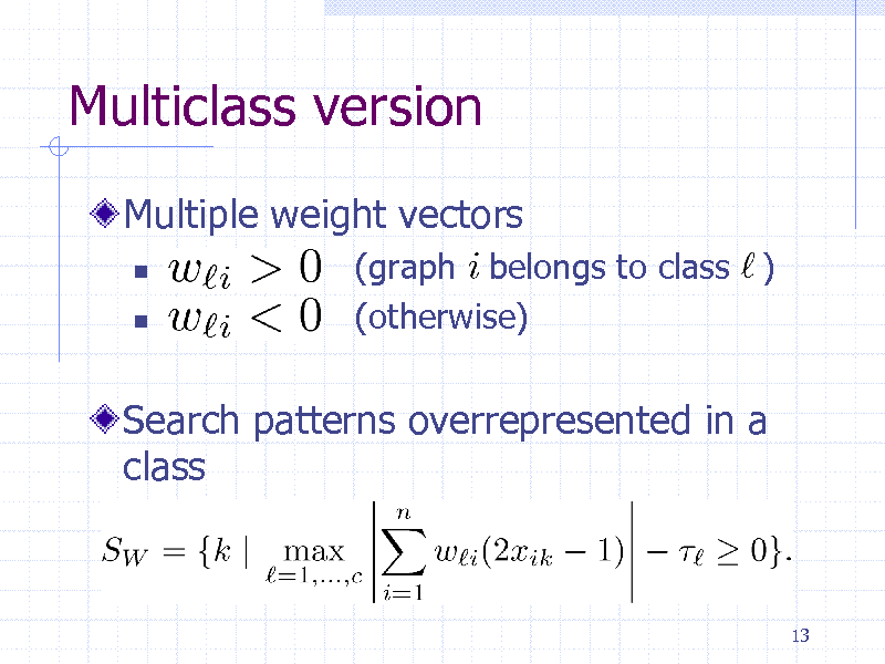
Multiclass version
Multiple weight vectors
(graph belongs to class ) (otherwise)
Search patterns overrepresented in a class
13
129
Basic Bound
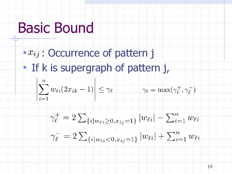
xij : Occurrence of pattern j If k is supergraph of pattern j,
14
130
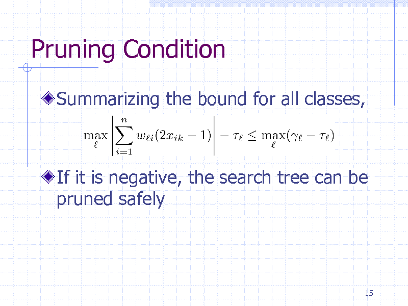
Pruning Condition
Summarizing the bound for all classes,
If it is negative, the search tree can be pruned safely
15
131
Summary: Preliminaries
Various graph learning problems
Supervised/Unsupervised
Discovery of salient features by graph mining Actual speed depends on the data
Faster for..
Sparse graphs Diverse kinds of labels
16
132
Part 2: EM-based clustering of graphs
17
133
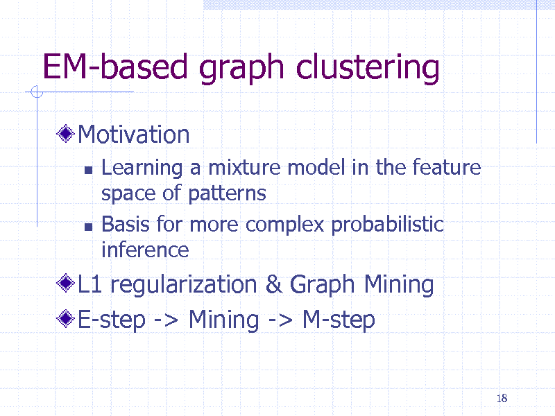
EM-based graph clustering
Motivation
Learning a mixture model in the feature space of patterns Basis for more complex probabilistic inference
L1 regularization & Graph Mining E-step -> Mining -> M-step
18
134
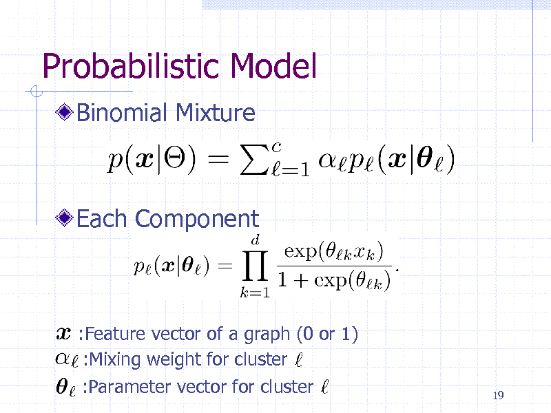
Probabilistic Model
Binomial Mixture
Each Component
:Feature vector of a graph (0 or 1) :Mixing weight for cluster :Parameter vector for cluster
19
135
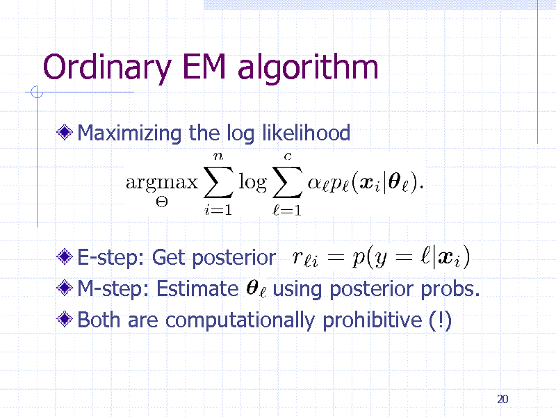
Ordinary EM algorithm
Maximizing the log likelihood
E-step: Get posterior M-step: Estimate using posterior probs. Both are computationally prohibitive (!)
20
136
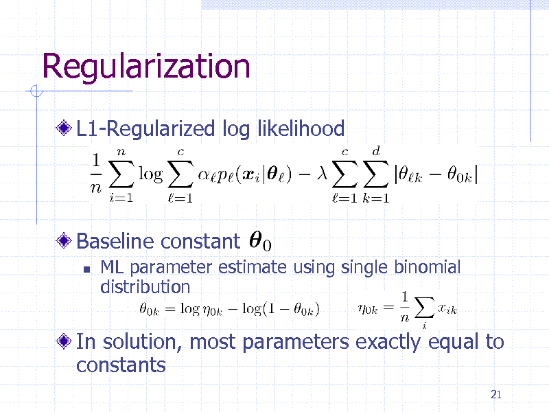
Regularization
L1-Regularized log likelihood
Baseline constant
ML parameter estimate using single binomial distribution
In solution, most parameters exactly equal to constants
21
137
E-step
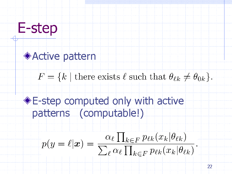
Active pattern
E-step computed only with active patterns (computable!)
22
138
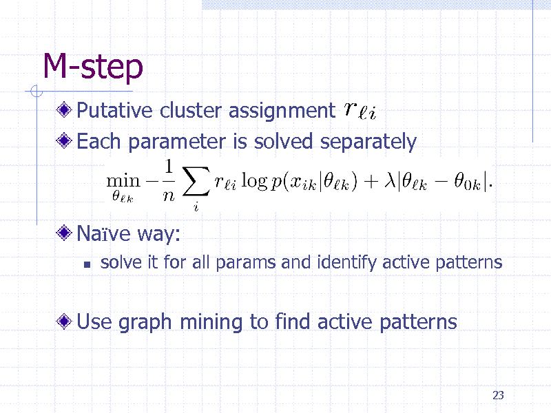
M-step
Putative cluster assignment Each parameter is solved separately
Nave way:
solve it for all params and identify active patterns
Use graph mining to find active patterns
23
139
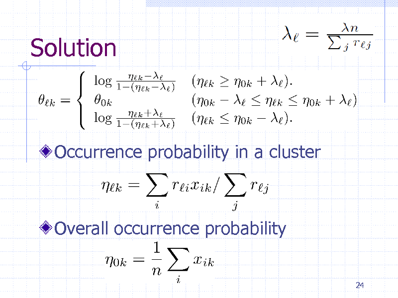
Solution
Occurrence probability in a cluster
Overall occurrence probability
24
140
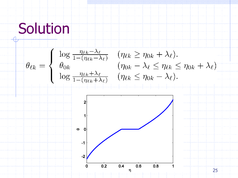
Solution
25
141
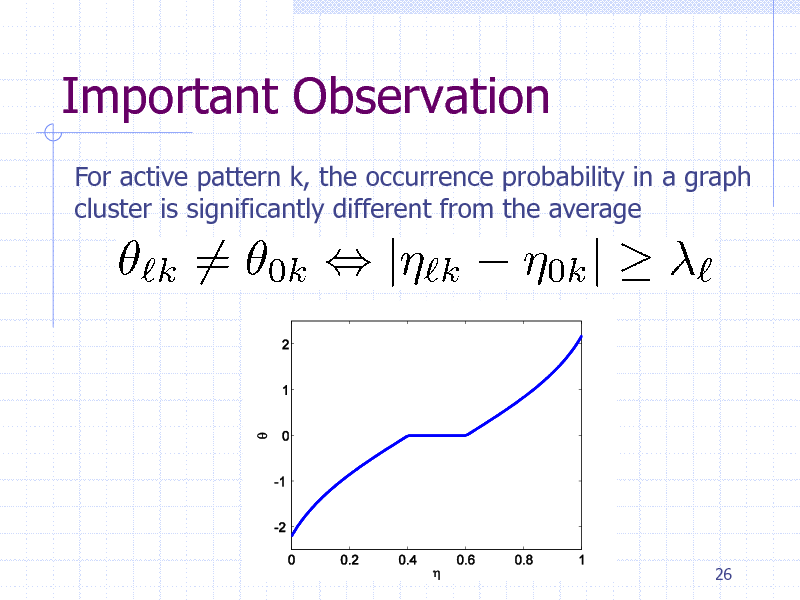
Important Observation
For active pattern k, the occurrence probability in a graph cluster is significantly different from the average
26
142
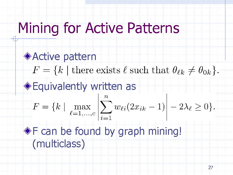
Mining for Active Patterns
Active pattern
Equivalently written as
F can be found by graph mining! (multiclass)
27
143
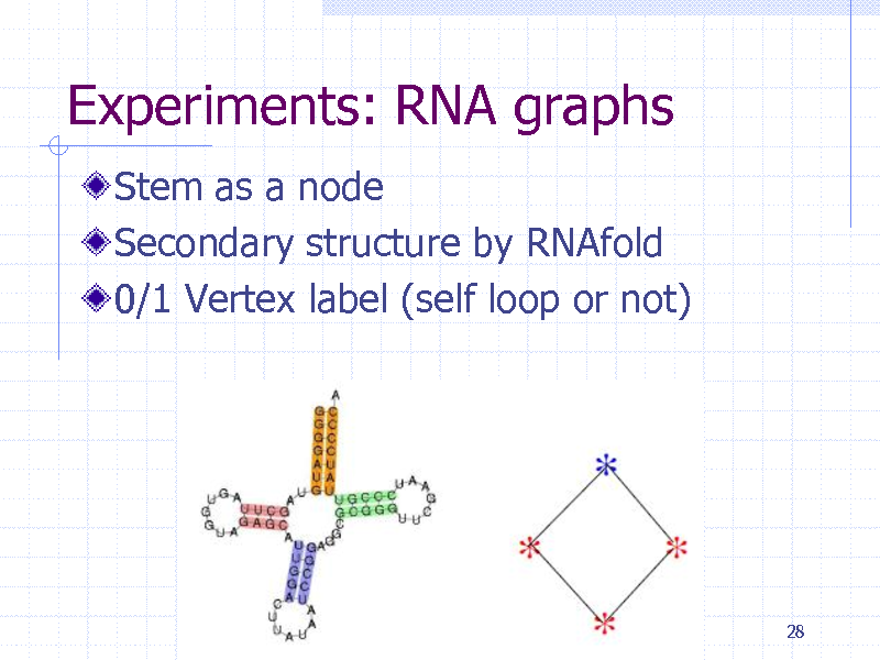
Experiments: RNA graphs
Stem as a node Secondary structure by RNAfold 0/1 Vertex label (self loop or not)
28
144
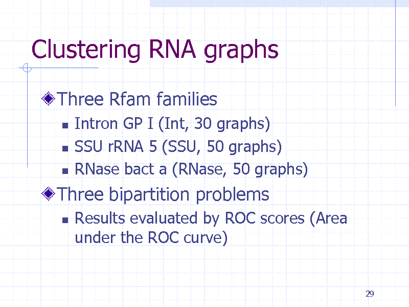
Clustering RNA graphs
Three Rfam families
Intron GP I (Int, 30 graphs) SSU rRNA 5 (SSU, 50 graphs) RNase bact a (RNase, 50 graphs)
Three bipartition problems
Results evaluated by ROC scores (Area under the ROC curve)
29
145
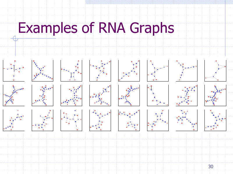
Examples of RNA Graphs
30
146
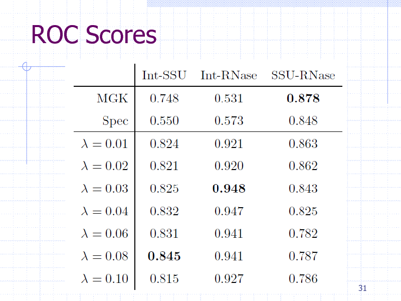
ROC Scores
31
147
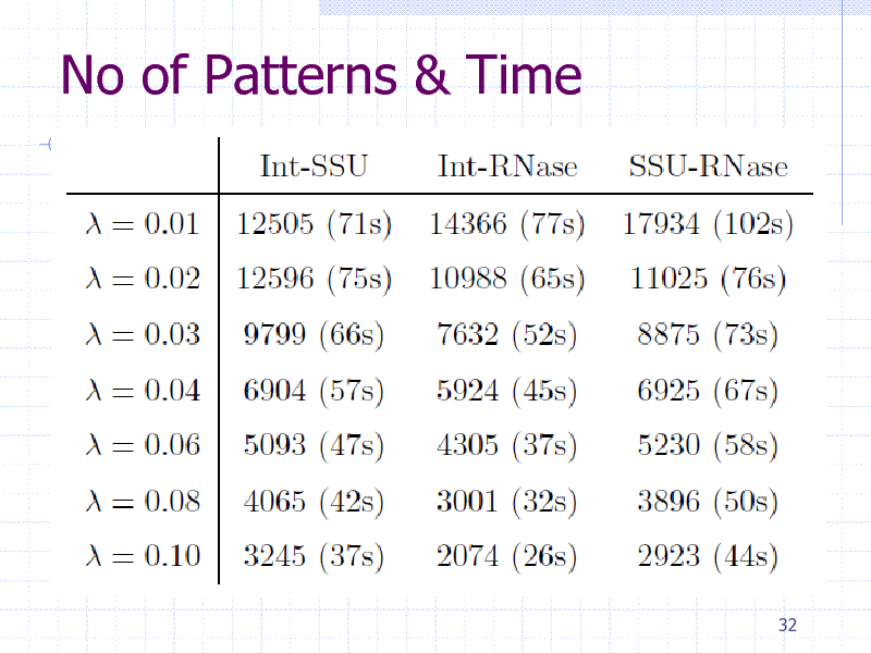
No of Patterns & Time
32
148
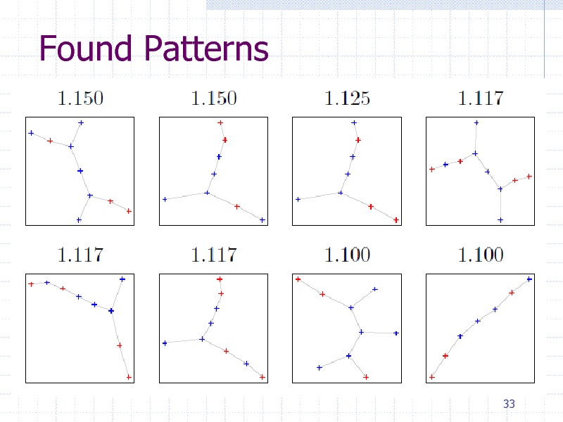
Found Patterns
33
149
Summary (graph EM)
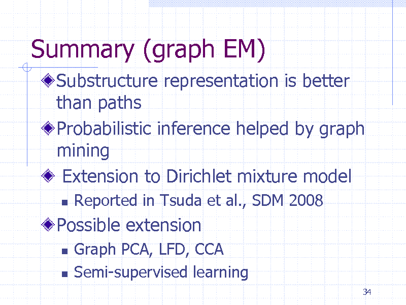
Substructure representation is better than paths Probabilistic inference helped by graph mining Extension to Dirichlet mixture model
Reported in Tsuda et al., SDM 2008 Graph PCA, LFD, CCA Semi-supervised learning
34
Possible extension
150

Part 3: Graph Boosting
35
151
Graph classification problem in chemoinformatics
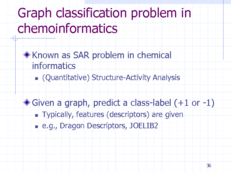
Known as SAR problem in chemical informatics
(Quantitative) Structure-Activity Analysis
Given a graph, predict a class-label (+1 or -1)
Typically, features (descriptors) are given e.g., Dragon Descriptors, JOELIB2
36
152

SAR with conventional descriptors
#atoms #bonds #rings 22 25
Activity +1
20 23
11 21
21 24
11 22
+1 +1
-1 -1
37
153
Motivation of Graph Boosting
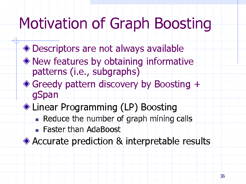
Descriptors are not always available New features by obtaining informative patterns (i.e., subgraphs) Greedy pattern discovery by Boosting + gSpan Linear Programming (LP) Boosting
Reduce the number of graph mining calls Faster than AdaBoost
Accurate prediction & interpretable results
38
154
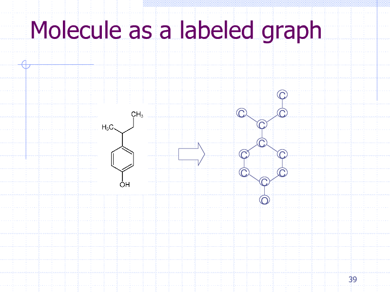
Molecule as a labeled graph
C C C C C C C O C C C
39
155
SAR with patterns
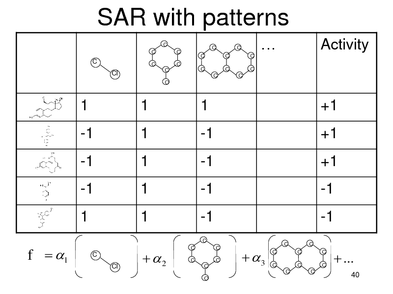
C C C C C O C C C C C C C C C C
Activity
C
C
Cl
1 -1 -1 -1 1
1 1 1 1 1
C Cl
1 -1 -1 -1 -1
C C C C O C C
+1 +1 +1 -1 -1
3
C C
f 1
2
C
C C
C
C C
C
C
...
40
156
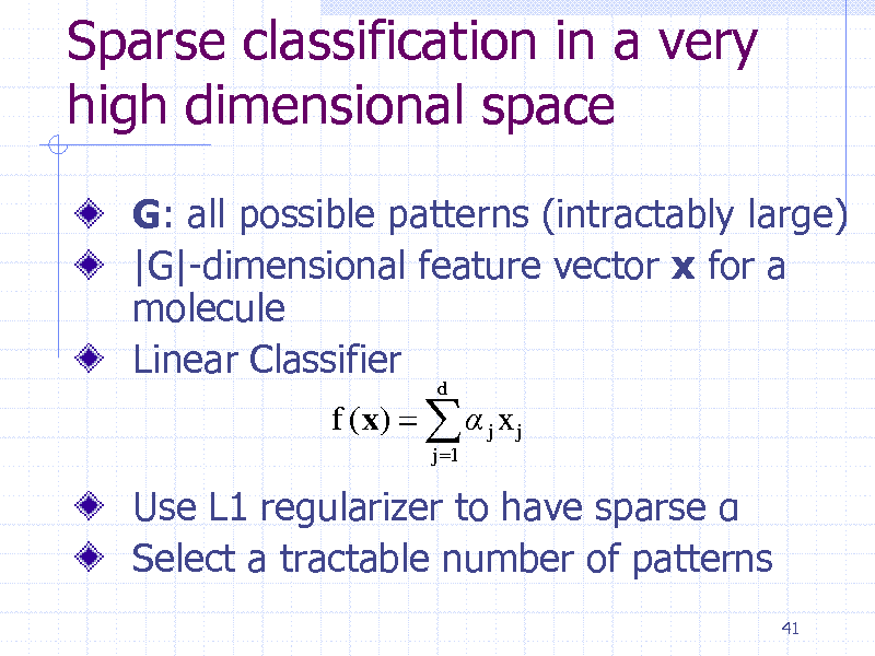
Sparse classification in a very high dimensional space
G: all possible patterns (intractably large) |G|-dimensional feature vector x for a molecule Linear Classifier
f (x) j x j
j 1 d
Use L1 regularizer to have sparse Select a tractable number of patterns
41
157
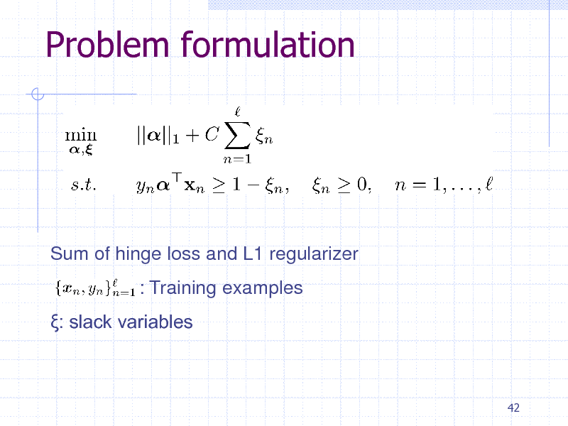
Problem formulation
Sum of hinge loss and L1 regularizer : Training examples : slack variables
42
158
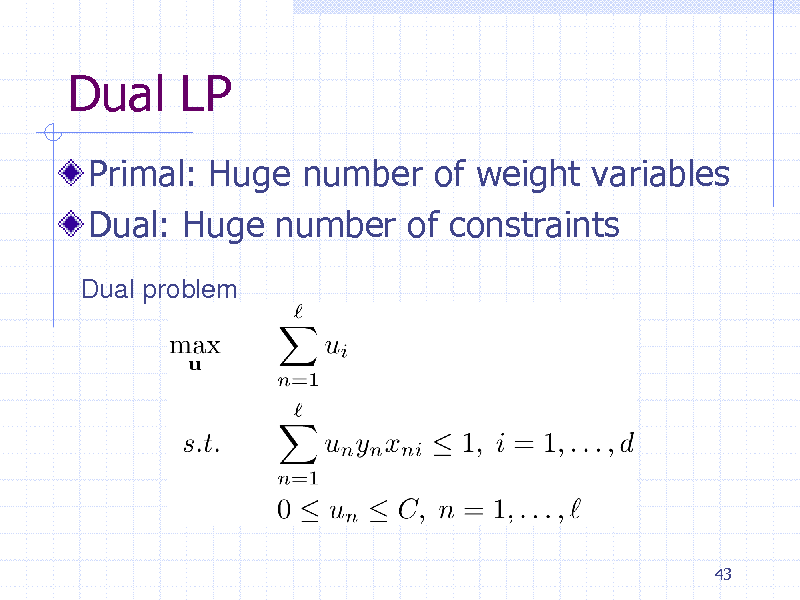
Dual LP
Primal: Huge number of weight variables Dual: Huge number of constraints
Dual problem
43
159
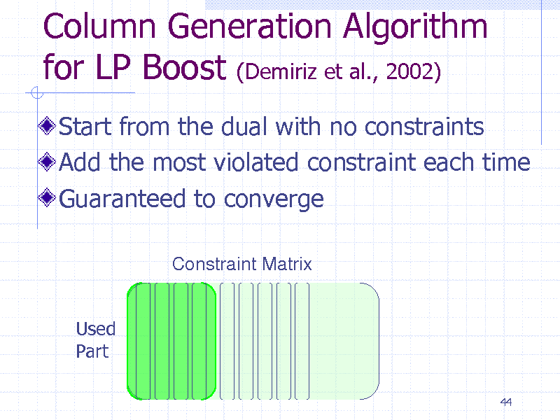
Column Generation Algorithm for LP Boost (Demiriz et al., 2002)
Start from the dual with no constraints Add the most violated constraint each time Guaranteed to converge
Constraint Matrix
Used Part
44
160
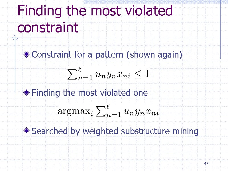
Finding the most violated constraint
Constraint for a pattern (shown again)
Finding the most violated one
Searched by weighted substructure mining
45
161
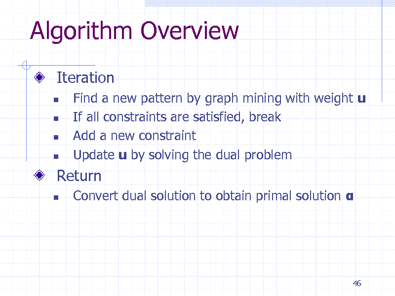
Algorithm Overview
Iteration
Find a new pattern by graph mining with weight u If all constraints are satisfied, break Add a new constraint Update u by solving the dual problem
Convert dual solution to obtain primal solution
Return
46
162
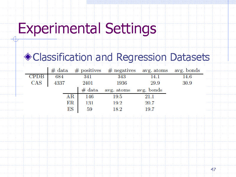
Experimental Settings
Classification and Regression Datasets
47
163
Classification Results
48
164
Regression Results
49
165
Extracted patterns from CPDB
50
166
Memory Usage
51
167
Runtime
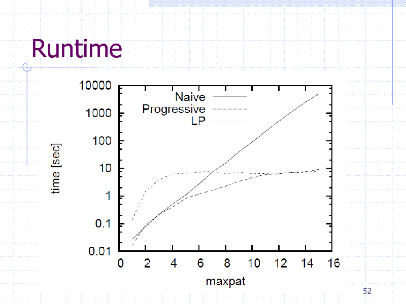
52
168
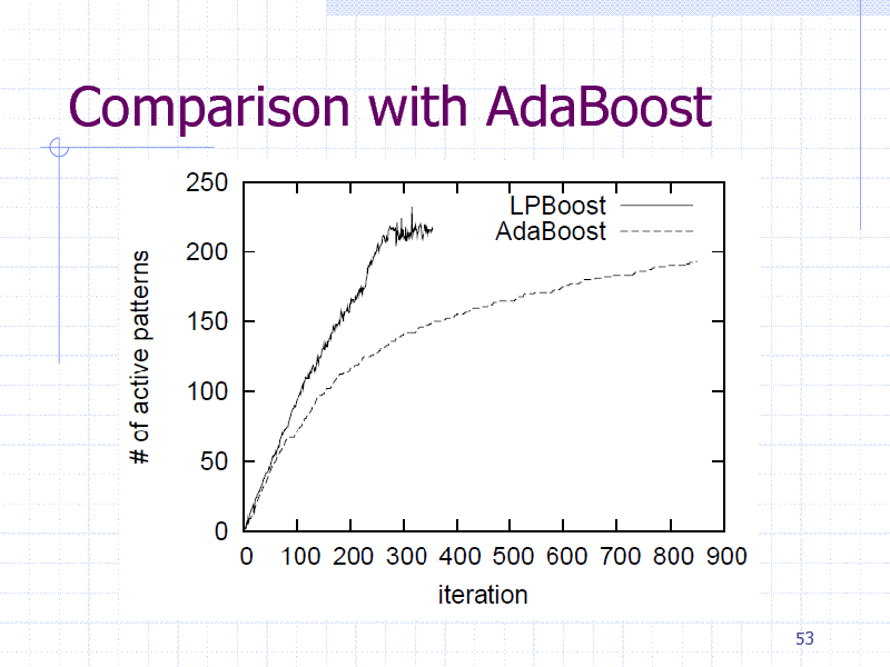
Comparison with AdaBoost
53
169
Summary (Graph Boosting)
Graph Boosting simultaneously generate patterns and learn their weights Finite convergence by column generation Interpretable by chemists. Flexible constraints and speed-up by LP.
54
170
Part 4: Entire Regularization Path
55
171
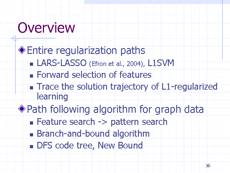
Overview
Entire regularization paths
LARS-LASSO (Efron et al., 2004), L1SVM Forward selection of features Trace the solution trajectory of L1-regularized learning Feature search -> pattern search Branch-and-bound algorithm DFS code tree, New Bound
56
Path following algorithm for graph data
172
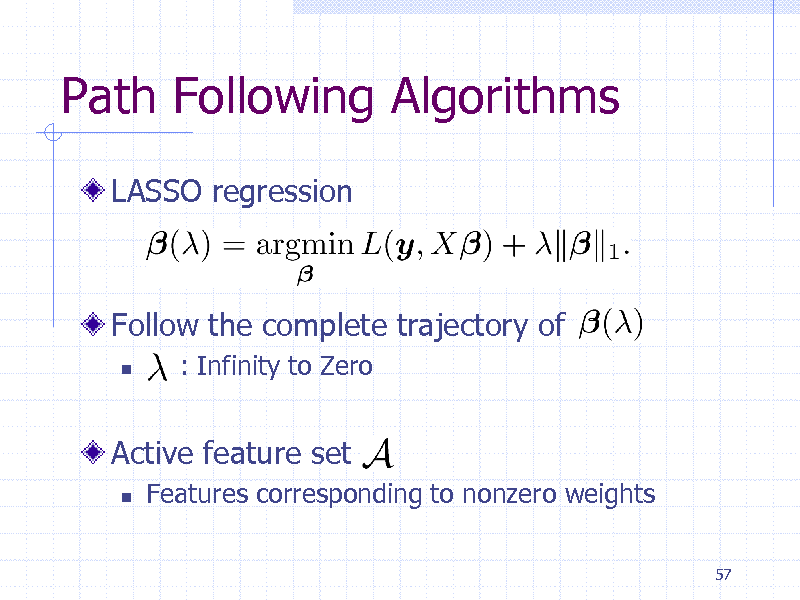
Path Following Algorithms
LASSO regression
Follow the complete trajectory of
: Infinity to Zero
Active feature set
Features corresponding to nonzero weights
57
173
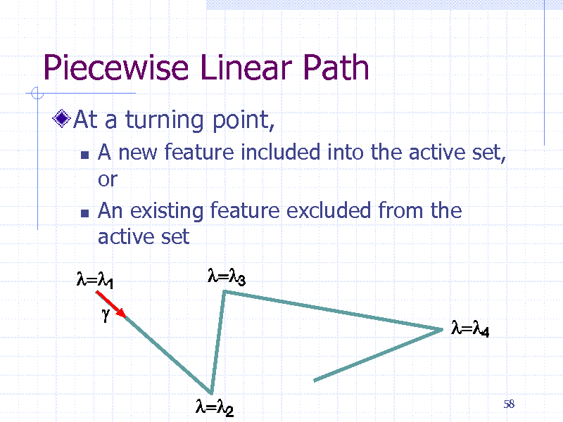
Piecewise Linear Path
At a turning point,
A new feature included into the active set, or An existing feature excluded from the active set
58
174
Practical Merit of Path Following
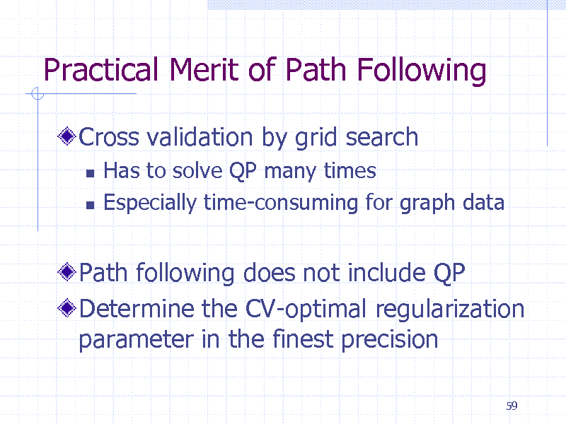
Cross validation by grid search
Has to solve QP many times Especially time-consuming for graph data
Path following does not include QP Determine the CV-optimal regularization parameter in the finest precision
59
175
Pseudo code of path following
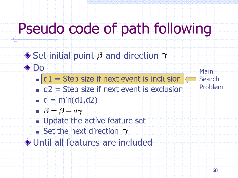
Set initial point Do
and direction
Main Search Problem
d1 = Step size if next event is inclusion d2 = Step size if next event is exclusion d = min(d1,d2) Update the active feature set Set the next direction
Until all features are included
60
176
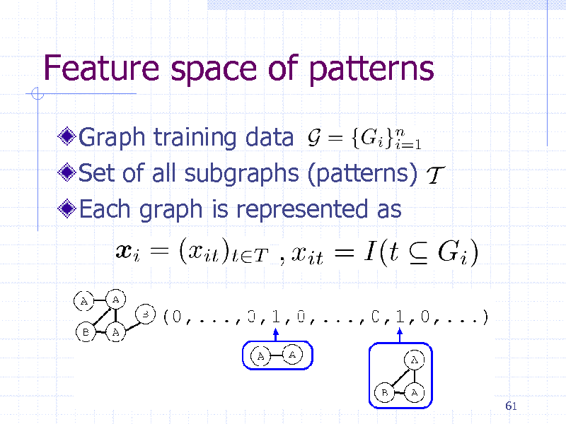
Feature space of patterns
Graph training data Set of all subgraphs (patterns) Each graph is represented as
61
177
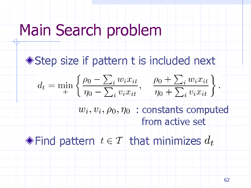
Main Search problem
Step size if pattern t is included next
: constants computed from active set
Find pattern
that minimizes
62
178
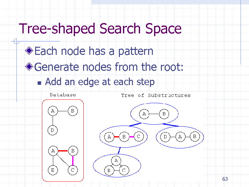
Tree-shaped Search Space
Each node has a pattern Generate nodes from the root:
Add an edge at each step
63
179

Tree Pruning
If it is guaranteed that the optimal pattern is not in the downstream, the search tree can be pruned
Not generated
64
180
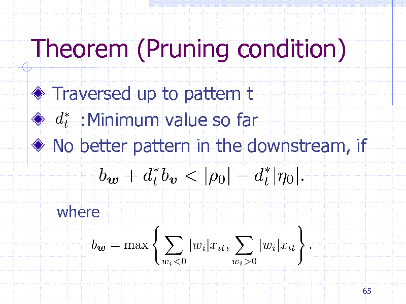
Theorem (Pruning condition)
Traversed up to pattern t :Minimum value so far No better pattern in the downstream, if
where
65
181
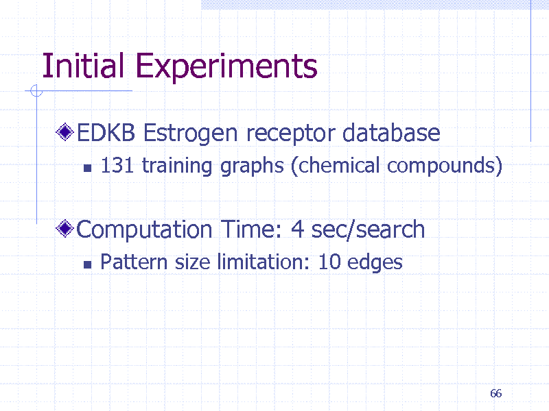
Initial Experiments
EDKB Estrogen receptor database
131 training graphs (chemical compounds)
Computation Time: 4 sec/search
Pattern size limitation: 10 edges
66
182
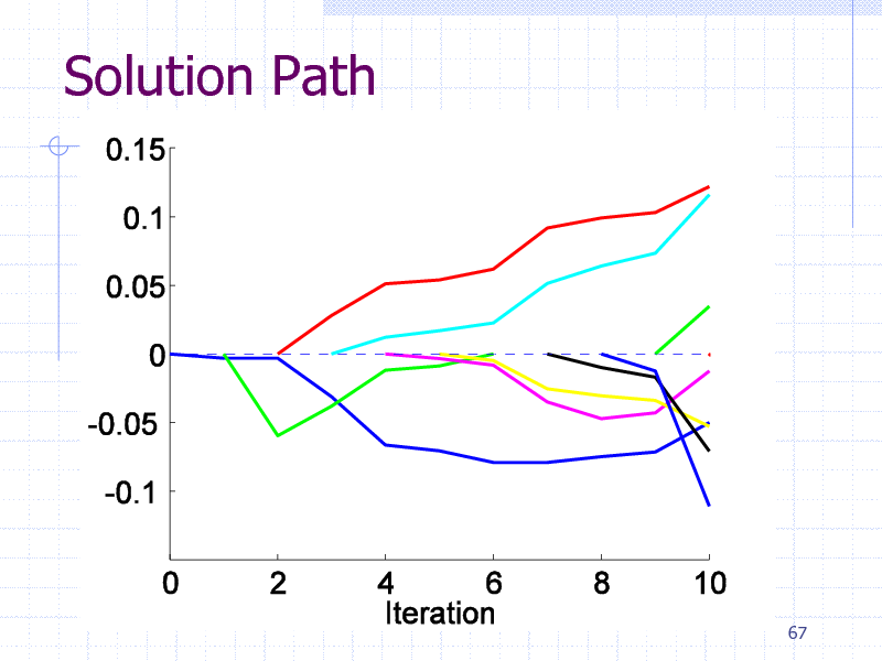
Solution Path
67
183
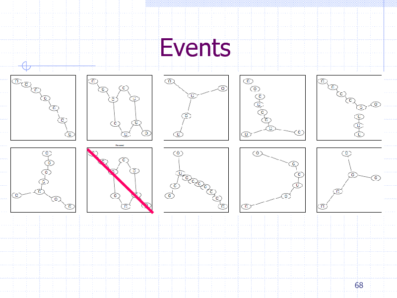
Events
68
184
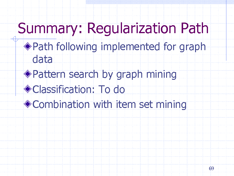
Summary: Regularization Path
Path following implemented for graph data Pattern search by graph mining Classification: To do Combination with item set mining
69
185
Part 5: . Itemset Boosting for predicting HIV drug resistance
70
186
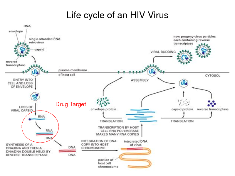
Life cycle of an HIV Virus
Drug Target
71
187
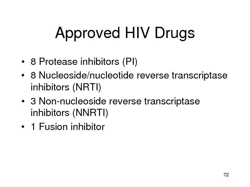
Approved HIV Drugs
8 Protease inhibitors (PI) 8 Nucleoside/nucleotide reverse transcriptase inhibitors (NRTI) 3 Non-nucleoside reverse transcriptase inhibitors (NNRTI) 1 Fusion inhibitor
72
188
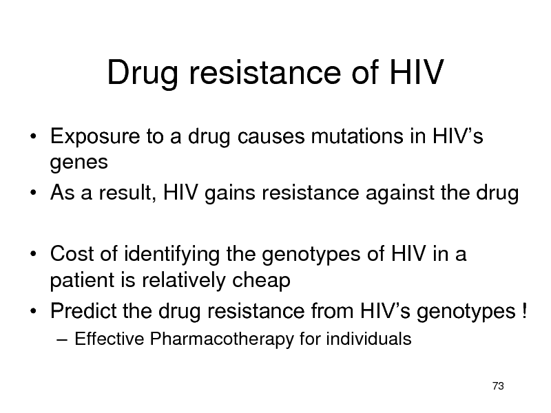
Drug resistance of HIV
Exposure to a drug causes mutations in HIVs genes As a result, HIV gains resistance against the drug
Cost of identifying the genotypes of HIV in a patient is relatively cheap Predict the drug resistance from HIVs genotypes !
Effective Pharmacotherapy for individuals
73
189
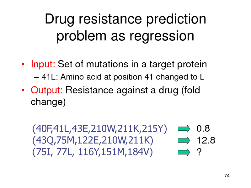
Drug resistance prediction problem as regression
Input: Set of mutations in a target protein
41L: Amino acid at position 41 changed to L
Output: Resistance against a drug (fold change) (40F,41L,43E,210W,211K,215Y) (43Q,75M,122E,210W,211K) (75I, 77L, 116Y,151M,184V) 0.8 12.8 ?
74
190
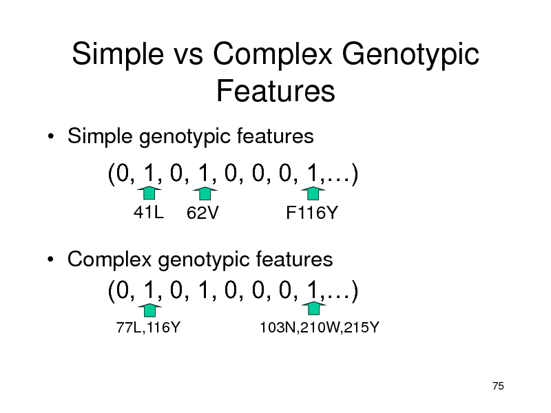
Simple vs Complex Genotypic Features
Simple genotypic features
(0, 1, 0, 1, 0, 0, 0, 1,)
41L
62V F116Y
Complex genotypic features
(0, 1, 0, 1, 0, 0, 0, 1,)
77L,116Y 103N,210W,215Y
75
191
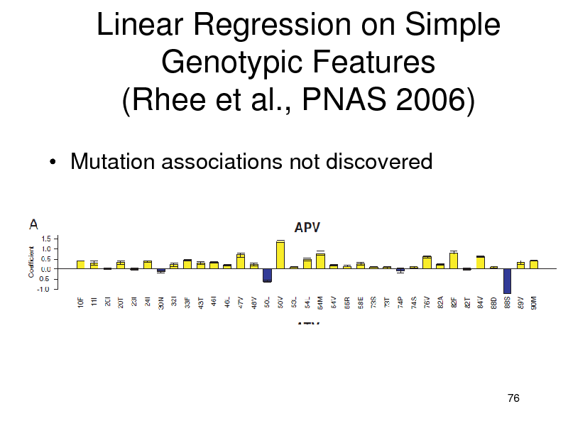
Linear Regression on Simple Genotypic Features (Rhee et al., PNAS 2006)
Mutation associations not discovered
76
192
Complex Genotypic Features
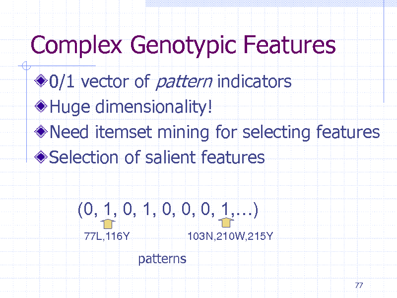
0/1 vector of pattern indicators Huge dimensionality! Need itemset mining for selecting features Selection of salient features (0, 1, 0, 1, 0, 0, 0, 1,)
77L,116Y 103N,210W,215Y
patterns
77
193
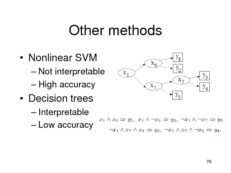
Other methods
Nonlinear SVM
Not interpretable High accuracy
Decision trees
Interpretable Low accuracy
78
194
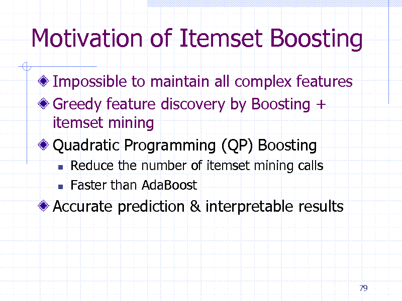
Motivation of Itemset Boosting
Impossible to maintain all complex features Greedy feature discovery by Boosting + itemset mining Quadratic Programming (QP) Boosting
Reduce the number of itemset mining calls Faster than AdaBoost
Accurate prediction & interpretable results
79
195
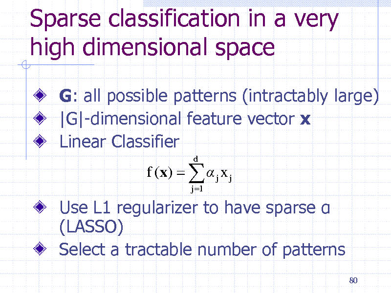
Sparse classification in a very high dimensional space
G: all possible patterns (intractably large) |G|-dimensional feature vector x Linear Classifier
f (x) j x j
j 1 d
Use L1 regularizer to have sparse (LASSO) Select a tractable number of patterns
80
196
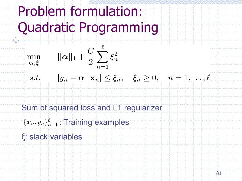
Problem formulation: Quadratic Programming
Sum of squared loss and L1 regularizer : Training examples : slack variables
81
197
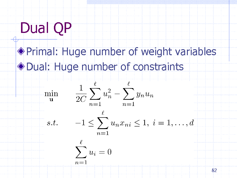
Dual QP
Primal: Huge number of weight variables Dual: Huge number of constraints
82
198
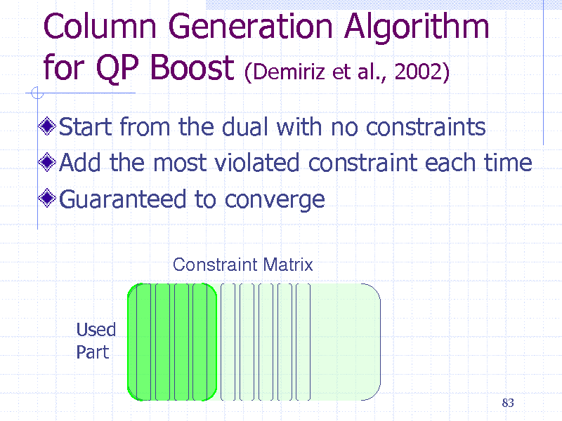
Column Generation Algorithm for QP Boost (Demiriz et al., 2002)
Start from the dual with no constraints Add the most violated constraint each time Guaranteed to converge
Constraint Matrix
Used Part
83
199
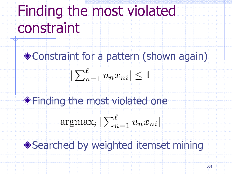
Finding the most violated constraint
Constraint for a pattern (shown again)
Finding the most violated one
Searched by weighted itemset mining
84
200

Algorithm Overview
Iteration
Find a new pattern by graph mining with weight u If all constraints are satisfied, break Add a new constraint Update u by solving the dual problem
Convert dual solution to obtain primal solution
Return
85
201
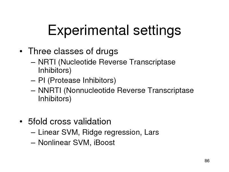
Experimental settings
Three classes of drugs
NRTI (Nucleotide Reverse Transcriptase Inhibitors) PI (Protease Inhibitors) NNRTI (Nonnucleotide Reverse Transcriptase Inhibitors)
5fold cross validation
Linear SVM, Ridge regression, Lars Nonlinear SVM, iBoost
86
202
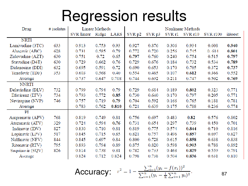
Regression results
Accuracy:
87
203
Accuracy Summary
NRTIs: iBoost performed best PIs:
Nonlinear methods were better than linear SVMs were slightly better (non-significant)
NNRTIs
Linear methods were better Combination is not necessary
88
204
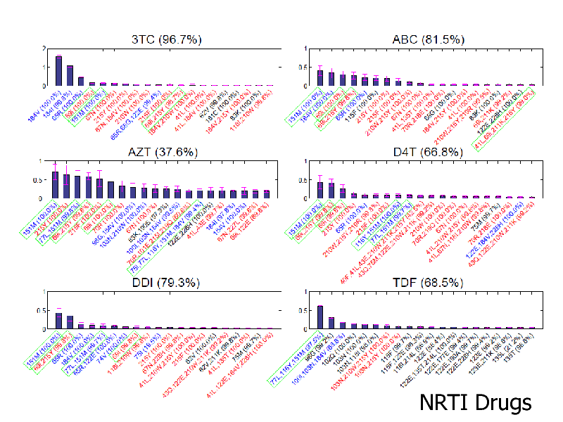
NRTI Drugs
89
205
Known mutation associations in RT
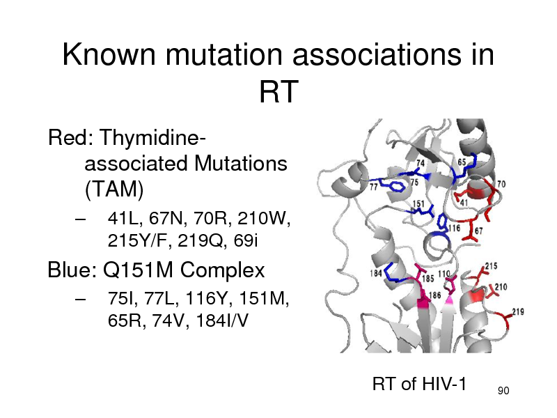
Red: Thymidineassociated Mutations (TAM)
41L, 67N, 70R, 210W, 215Y/F, 219Q, 69i 75I, 77L, 116Y, 151M, 65R, 74V, 184I/V
RT of HIV-1
Blue: Q151M Complex
90
206
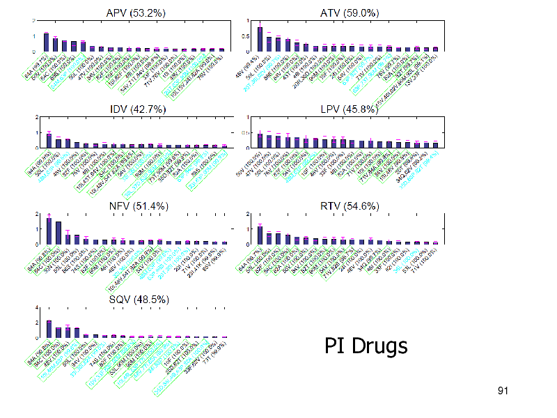
PI Drugs
91
207
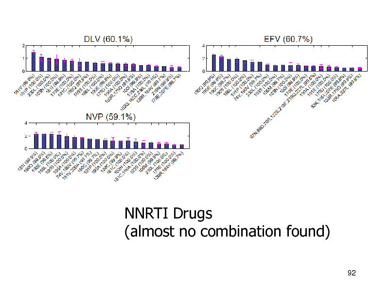
NNRTI Drugs (almost no combination found)
92
208
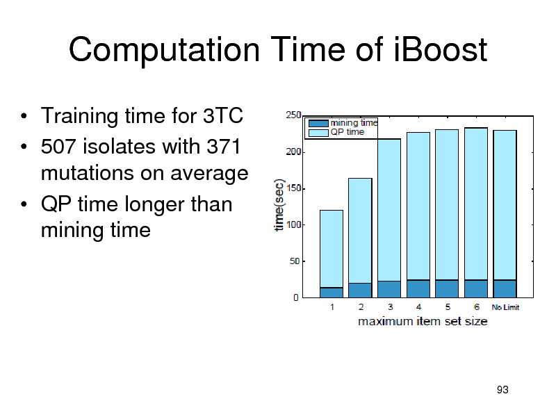
Computation Time of iBoost
Training time for 3TC 507 isolates with 371 mutations on average QP time longer than mining time
93
209
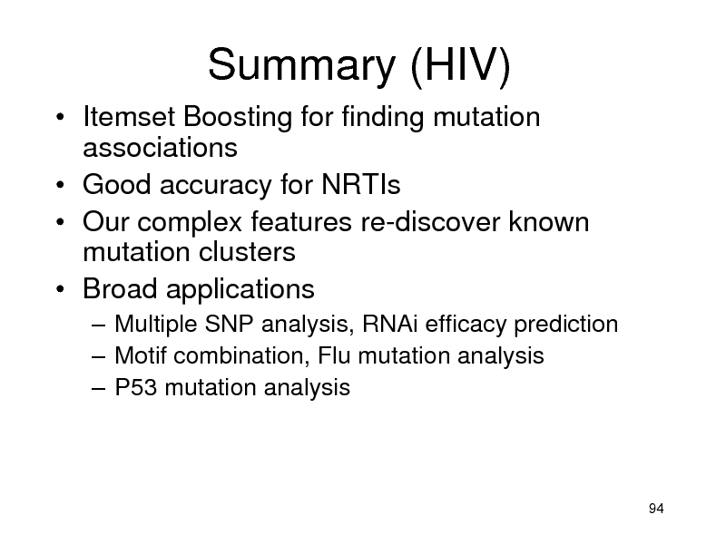
Summary (HIV)
Itemset Boosting for finding mutation associations Good accuracy for NRTIs Our complex features re-discover known mutation clusters Broad applications
Multiple SNP analysis, RNAi efficacy prediction Motif combination, Flu mutation analysis P53 mutation analysis
94
210
![Slide: Reference
[1] K. Tsuda and T. Kudo, Clustering graphs by weighted substructure mining, in Proceedings of the 23rd international conference on Machine learning - ICML 06, 2006, pp. 953960. [2] H. Saigo, N. Krmer, and K. Tsuda, Partial least squares regression for graph mining, in Proceeding of the 14th ACM SIGKDD international conference on Knowledge discovery and data mining - KDD 08, 2008, p. 578. [3] H. Saigo, S. Nowozin, T. Kadowaki, T. Kudo, and K. Tsuda, gBoost: a mathematical programming approach to graph classification and regression, Machine Learning, vol. 75, no. 1, pp. 6989, Nov. 2008. [4] H. Saigo, T. Uno, and K. Tsuda, Mining complex genotypic features for predicting HIV-1 drug resistance., Bioinformatics (Oxford, England), vol. 23, no. 18, pp. 245562, Sep. 2007. [5] K. Tsuda, Entire regularization paths for graph data, in Proceedings of the 24th international conference on Machine learning - ICML 07, 2007, pp. 919926.
95](https://yosinski.com/mlss12/media/slides/MLSS-2012-Tsuda-Graph-Mining_211.png)
Reference
[1] K. Tsuda and T. Kudo, Clustering graphs by weighted substructure mining, in Proceedings of the 23rd international conference on Machine learning - ICML 06, 2006, pp. 953960. [2] H. Saigo, N. Krmer, and K. Tsuda, Partial least squares regression for graph mining, in Proceeding of the 14th ACM SIGKDD international conference on Knowledge discovery and data mining - KDD 08, 2008, p. 578. [3] H. Saigo, S. Nowozin, T. Kadowaki, T. Kudo, and K. Tsuda, gBoost: a mathematical programming approach to graph classification and regression, Machine Learning, vol. 75, no. 1, pp. 6989, Nov. 2008. [4] H. Saigo, T. Uno, and K. Tsuda, Mining complex genotypic features for predicting HIV-1 drug resistance., Bioinformatics (Oxford, England), vol. 23, no. 18, pp. 245562, Sep. 2007. [5] K. Tsuda, Entire regularization paths for graph data, in Proceedings of the 24th international conference on Machine learning - ICML 07, 2007, pp. 919926.
95
211
Machine Learning Summer School Kyoto 2012
Graph Mining
Chapter 3: Kernels for Structured Data
National Institute of Advanced Industrial Science and Technology Koji Tsuda
1
212
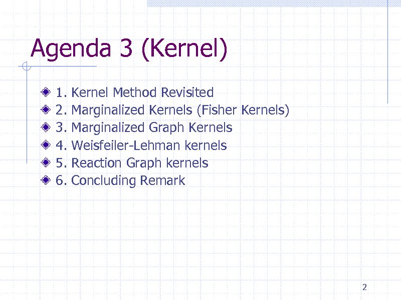
Agenda 3 (Kernel)
1. 2. 3. 4. 5. 6. Kernel Method Revisited Marginalized Kernels (Fisher Kernels) Marginalized Graph Kernels Weisfeiler-Lehman kernels Reaction Graph kernels Concluding Remark
2
213

Part 1: Kernel Method Revisited
3
214
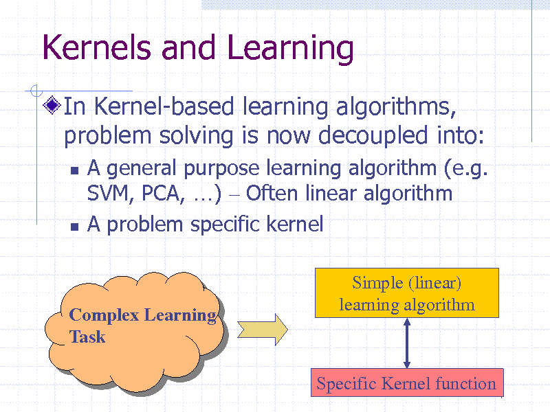
Kernels and Learning
In Kernel-based learning algorithms, problem solving is now decoupled into:
A general purpose learning algorithm (e.g. SVM, PCA, ) Often linear algorithm A problem specific kernel
Simple (linear) learning algorithm
Complex Learning Task
Specific Kernel function 4
215
Current Synthesis
Modularity and re-usability
Same kernel ,different learning algorithms Different kernels, same learning algorithms
Data 1 (Sequence) Data 2 (Network)
Kernel 1
Gram Matrix
(not necessarily stored)
Learning Algo 1 Learning Algo 2
5
Kernel 2 Gram Matrix
216
Kernel Methods : intuitive idea
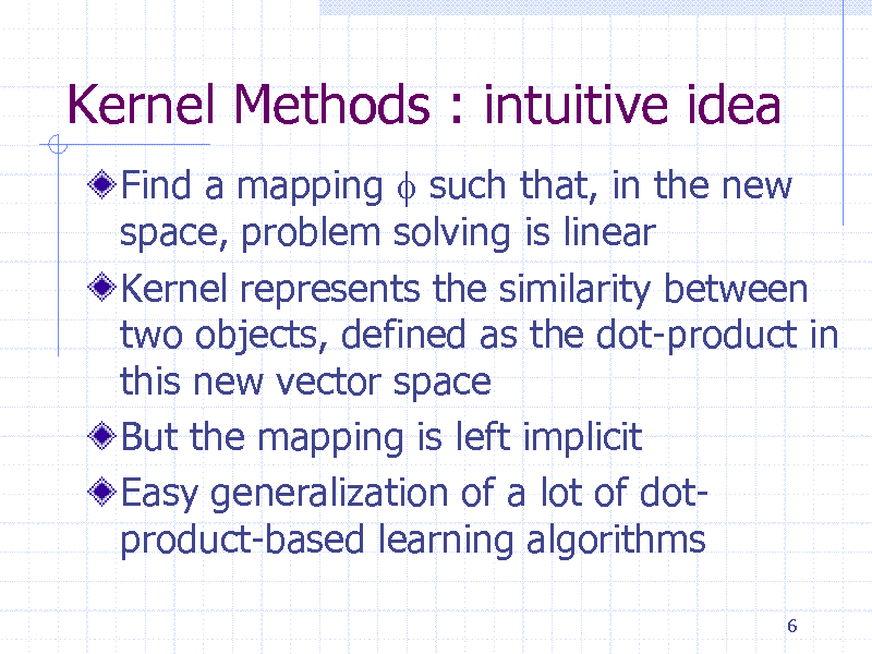
Find a mapping f such that, in the new space, problem solving is linear Kernel represents the similarity between two objects, defined as the dot-product in this new vector space But the mapping is left implicit Easy generalization of a lot of dotproduct-based learning algorithms
6
217
Kernel Methods : the mapping
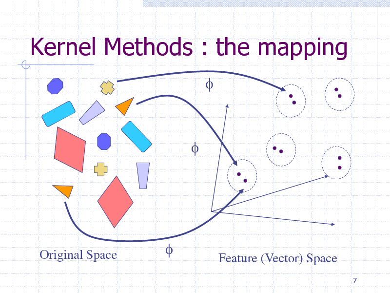
f
f
Original Space
f
Feature (Vector) Space
7
218
Kernel : more formal definition
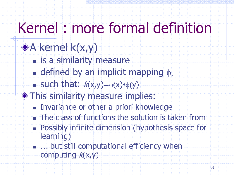
A kernel k(x,y)
is a similarity measure defined by an implicit mapping f, such that: k(x,y)=f(x)f(y) This similarity measure implies:
Invariance or other a priori knowledge The class of functions the solution is taken from Possibly infinite dimension (hypothesis space for learning) but still computational efficiency when computing k(x,y)
8
219
Kernel Trick
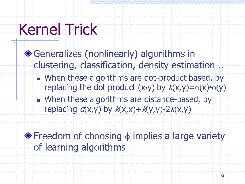
Generalizes (nonlinearly) algorithms in clustering, classification, density estimation ..
When these algorithms are dot-product based, by replacing the dot product (xy) by k(x,y)=f(x)f(y) When these algorithms are distance-based, by replacing d(x,y) by k(x,x)+k(y,y)-2k(x,y)
Freedom of choosing f implies a large variety of learning algorithms
9
220
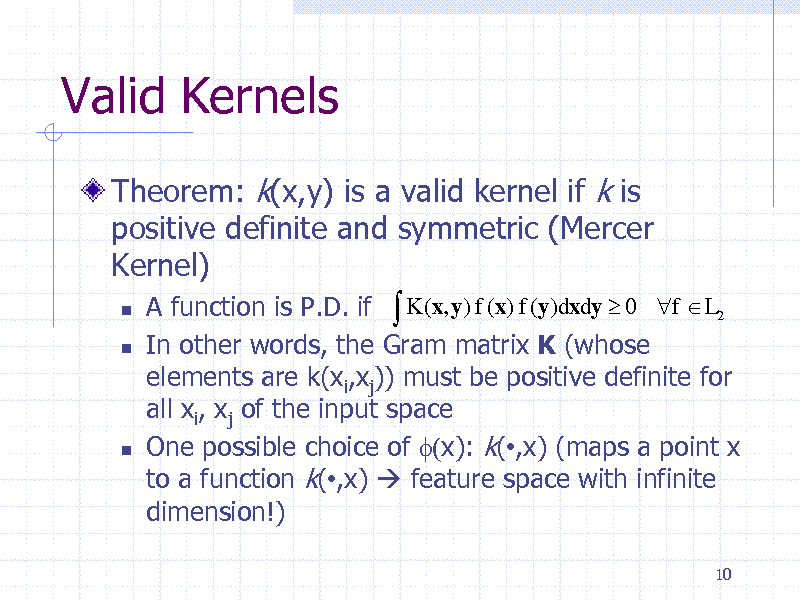
Valid Kernels
Theorem: k(x,y) is a valid kernel if k is positive definite and symmetric (Mercer Kernel)
A function is P.D. if K (x, y) f (x) f (y)dxdy 0 f L2 In other words, the Gram matrix K (whose elements are k(xi,xj)) must be positive definite for all xi, xj of the input space One possible choice of f(x): k(,x) (maps a point x to a function k(,x) feature space with infinite dimension!)
10
221
How to build new kernels
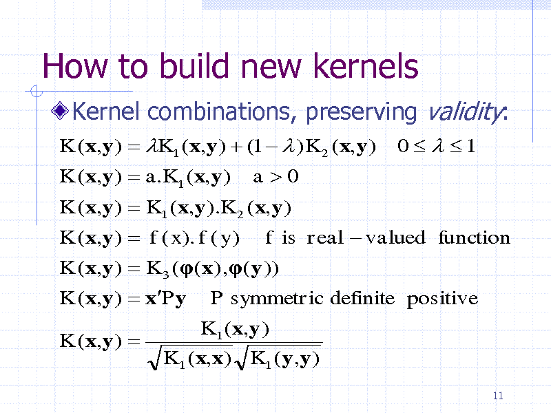
Kernel combinations, preserving validity:
K (x,y ) K1 ( x,y ) (1 ) K 2 (x,y ) K (x,y ) a.K1 (x,y ) a0 K (x,y ) K1 ( x,y ).K 2 ( x,y ) K (x,y ) f ( x). f ( y ) f is real valued function K (x,y ) K 3 (( x) ,(y )) K (x,y ) xPy P symmetric definite positive K (x,y ) K1 ( x,y ) K1 ( x,x) K1 (y,y )
11
0 1
222

Strategies of Design
Convolution Kernels: text is a recursively-defined data structure. How to build global kernels form local (atomic level) kernels? Generative model-based kernels: the topology of the problem will be translated into a kernel function
12
223
IBM Research Tokyo Research Laboratory
2005 IBM Corporation
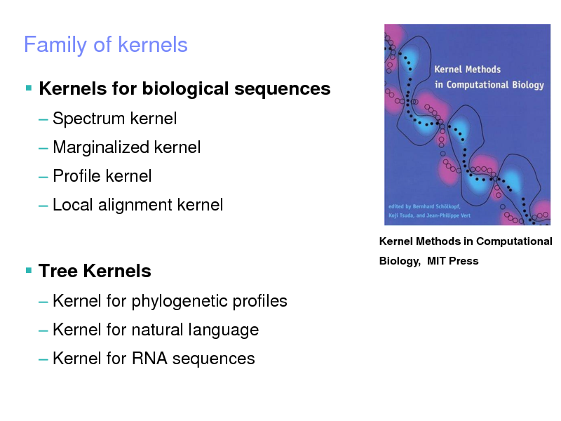
Family of kernels
Kernels for biological sequences
Spectrum kernel Marginalized kernel Profile kernel Local alignment kernel
Kernel Methods in Computational Biology, MIT Press
Tree Kernels
Kernel for phylogenetic profiles
Kernel for natural language Kernel for RNA sequences
224
IBM Research Tokyo Research Laboratory
2005 IBM Corporation
Family of kernels
Kernels for nodes in a network
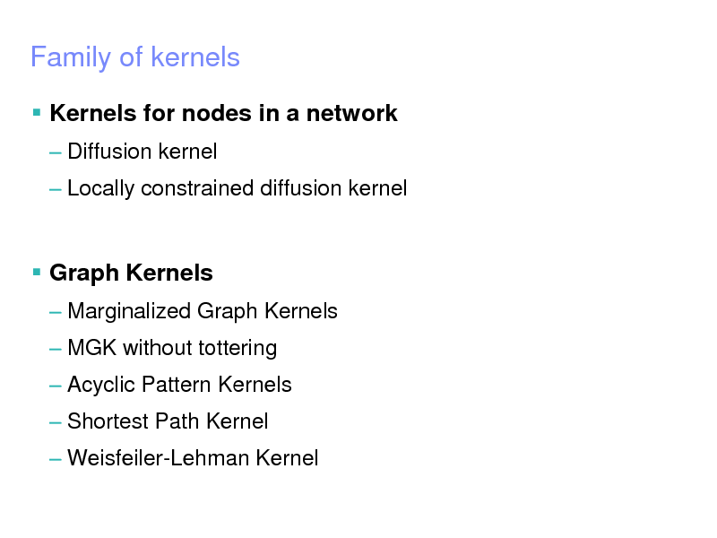
Diffusion kernel Locally constrained diffusion kernel
Graph Kernels
Marginalized Graph Kernels MGK without tottering
Acyclic Pattern Kernels
Shortest Path Kernel Weisfeiler-Lehman Kernel
225
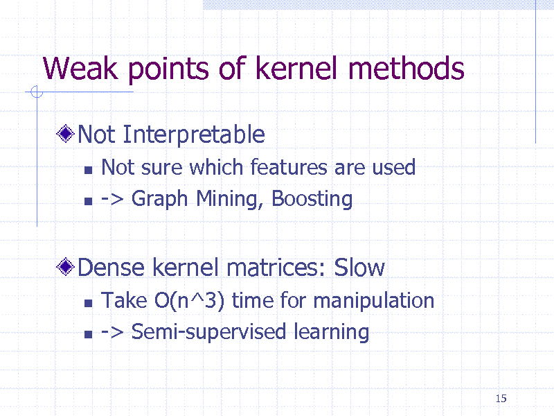
Weak points of kernel methods
Not Interpretable
Not sure which features are used -> Graph Mining, Boosting
Dense kernel matrices: Slow
Take O(n^3) time for manipulation -> Semi-supervised learning
15
226
Part 2. Marginalized kernels
16
227
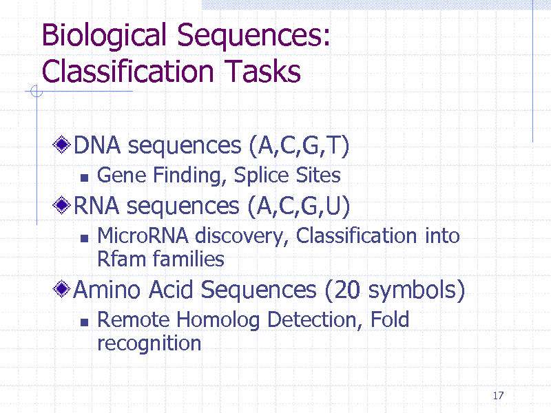
Biological Sequences: Classification Tasks
DNA sequences (A,C,G,T)
Gene Finding, Splice Sites MicroRNA discovery, Classification into Rfam families Remote Homolog Detection, Fold recognition
17
RNA sequences (A,C,G,U)
Amino Acid Sequences (20 symbols)
228
Kernels for Sequences
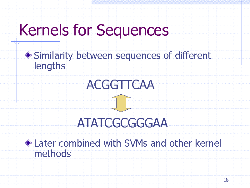
Similarity between sequences of different lengths
ACGGTTCAA ATATCGCGGGAA
Later combined with SVMs and other kernel methods
18
229
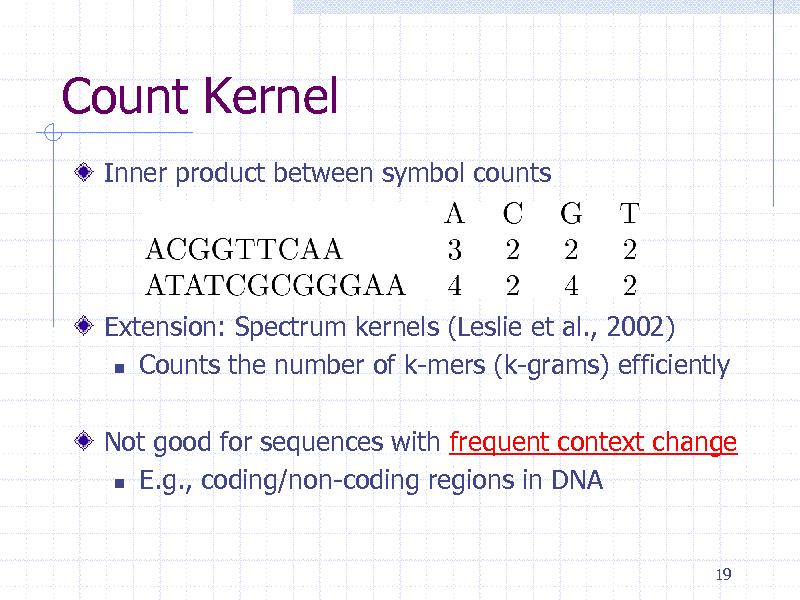
Count Kernel
Inner product between symbol counts
Extension: Spectrum kernels (Leslie et al., 2002) Counts the number of k-mers (k-grams) efficiently Not good for sequences with frequent context change E.g., coding/non-coding regions in DNA
19
230
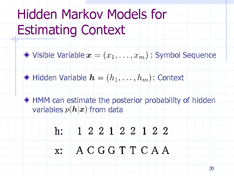
Hidden Markov Models for Estimating Context
Visible Variable
Hidden Variable
: Symbol Sequence
: Context
HMM can estimate the posterior probability of hidden variables from data
20
231
Marginalized kernels
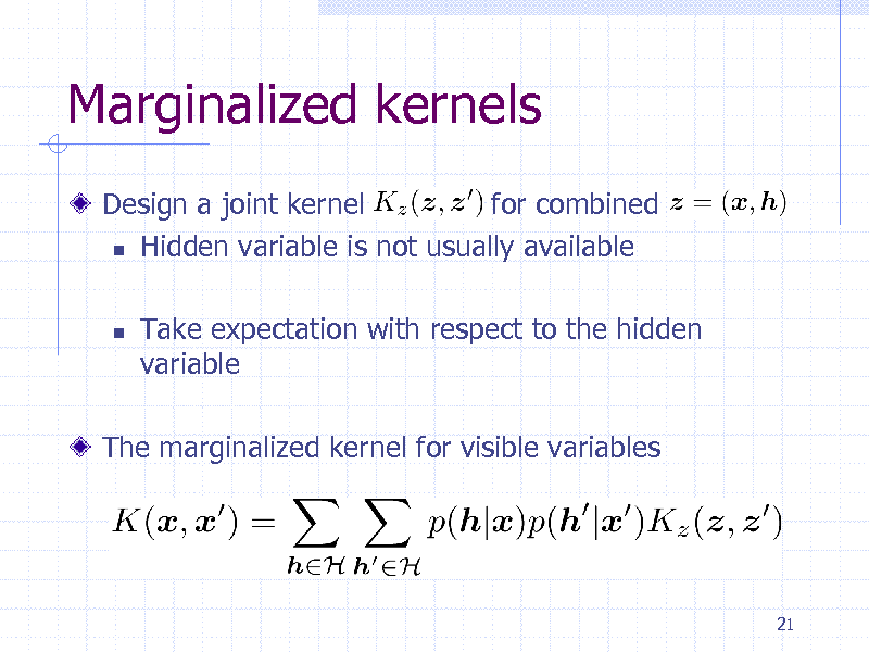
Design a joint kernel for combined Hidden variable is not usually available
Take expectation with respect to the hidden variable
The marginalized kernel for visible variables
21
232
Designing a joint kernel for sequences
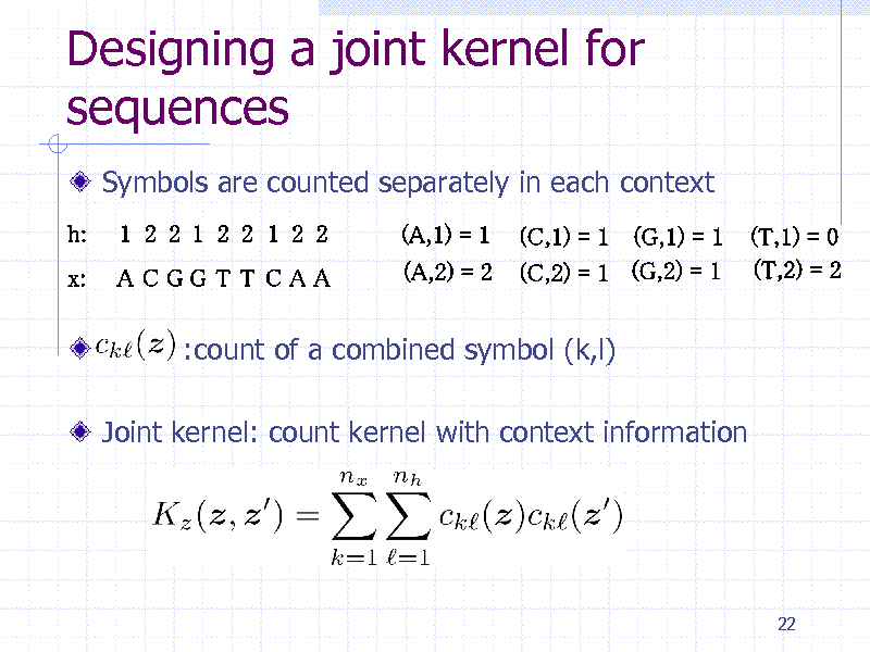
Symbols are counted separately in each context
:count of a combined symbol (k,l) Joint kernel: count kernel with context information
22
233
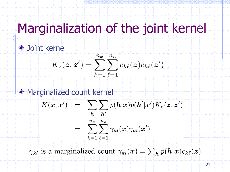
Marginalization of the joint kernel
Joint kernel
Marginalized count kernel
23
234
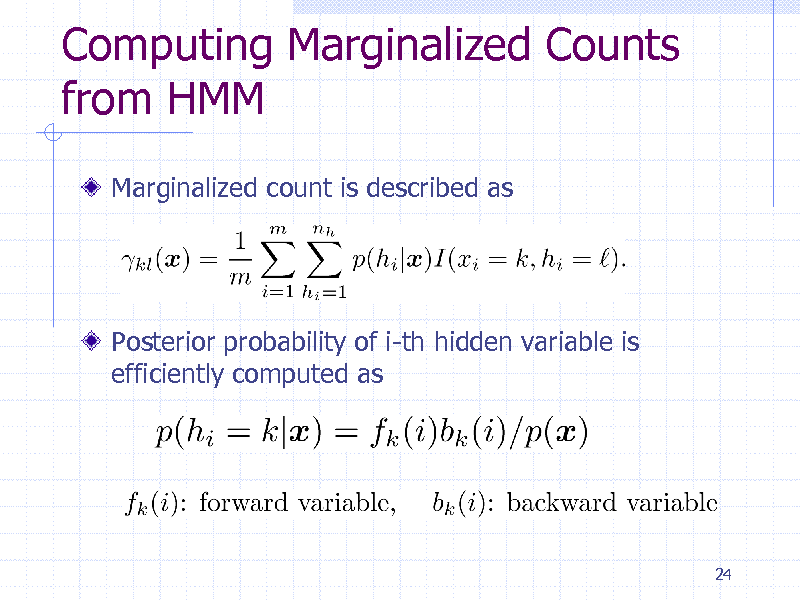
Computing Marginalized Counts from HMM
Marginalized count is described as
Posterior probability of i-th hidden variable is efficiently computed as
24
235
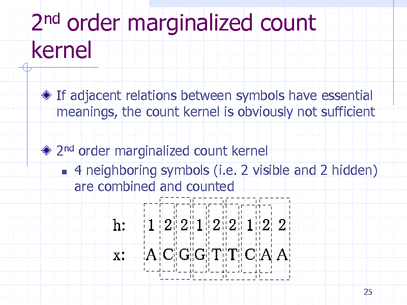
2nd order marginalized count kernel
If adjacent relations between symbols have essential meanings, the count kernel is obviously not sufficient
2nd order marginalized count kernel 4 neighboring symbols (i.e. 2 visible and 2 hidden) are combined and counted
25
236

Fisher Kernel
Probabilistic mode
Fisher Kernel Mapping to a feature vector (Fisher score vector)
Inner product of Fisher scores
Z: Fisher information matrix
26
237
Fisher Kernel from HMM
Derive FK from HMM (Jaakkola et al. 2000)
Derivative for emission probabilities only No Fisher information matrix Counts are centralized and weighted
FK from HMM is a special case of marginalized kernels
27
238
Difference between FK and Marginalized Kernels
FK: Probabilistic model determines the joint kernel and the posterior probabilities
MK: You can determine them separately
More flexible design!
28
239
Protein clustering experiment
84 proteins containing five classes
gyrB proteins from five bacteria species HMM + {FK,MCK1,MCK2}+K-Means
Clustering methods
Evaluation
Adjusted Rand Index (ARI)
29
240
Kernel Matrices
30
241
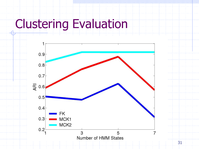
Clustering Evaluation
31
242
Applications since then..
Marginalized Graph Kernels (Kashima et al., ICML 2003) Sensor networks (Nyugen et al., ICML 2004) Labeling of structured data (Kashima et al., ICML 2004) Robotics (Shimosaka et al., ICRA 2005) Kernels for Promoter Regions (Vert et al., NIPS 2005) Web data (Zhao et al., WWW 2006)
32
243
Summary (Marginalized Kernels)
General Framework for using generative model for defining kernels Fisher kernel as a special case Broad applications
33
244

Part 3 Marginalized Graph Kernels
34
245
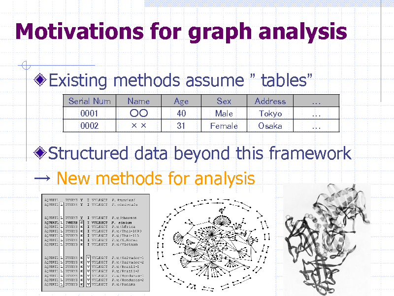
Motivations for graph analysis
Existing methods assume tables
Serial Num 0001 0002 Name Age 40 31 Sex Male Female Address Tokyo Osaka
Structured data beyond this framework New methods for analysis
35
246
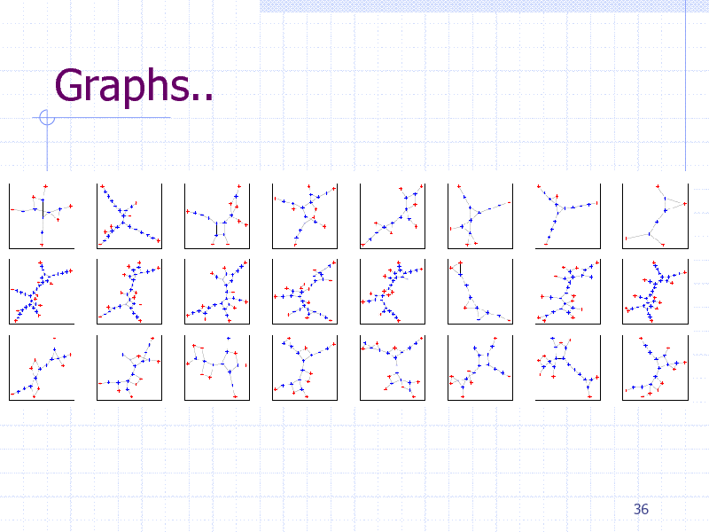
Graphs..
36
247
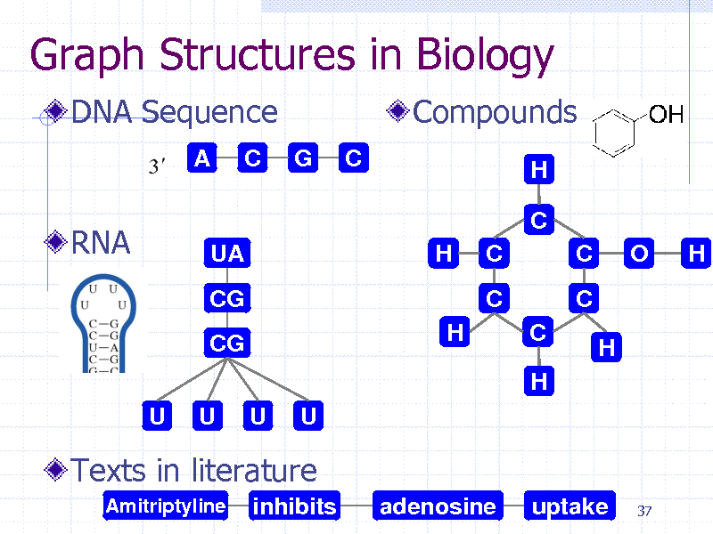
Graph Structures in Biology
DNA Sequence
A C G C
Compounds
H
RNA
C
UA CG CG U U U U H H C C O H
C
C H
C
H
Texts in literature
Amitriptyline
inhibits
adenosine
uptake
37
248
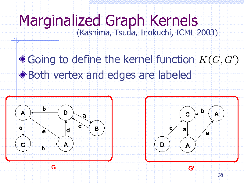
Marginalized Graph Kernels
Going to define the kernel function Both vertex and edges are labeled
(Kashima, Tsuda, Inokuchi, ICML 2003)
38
249
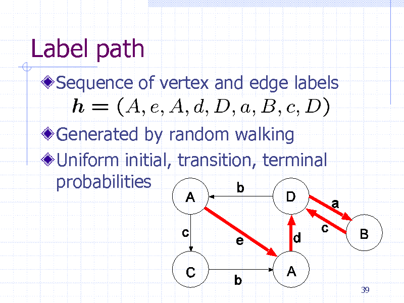
Label path
Sequence of vertex and edge labels
Generated by random walking Uniform initial, transition, terminal probabilities
39
250
Path-probability vector
40
251
Kernel definition
Kernels for paths
A c D b E
B c D a A
Take expectation over all possible paths! Marginalized kernels for graphs
41
252
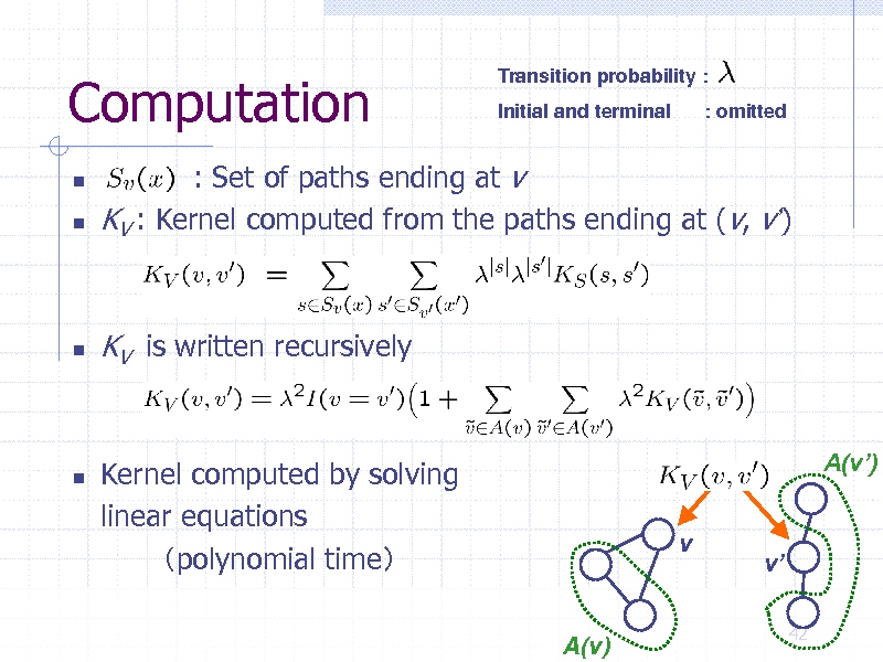
Computation
Transition probability : Initial and terminal : omitted
: Set of paths ending at v KV : Kernel computed from the paths ending at (v, v)
KV is written recursively
Kernel computed by solving linear equations polynomial time
A(v)
A(v) v
v
42
253
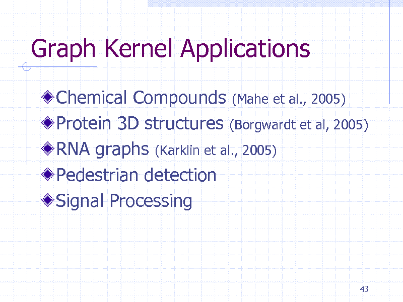
Graph Kernel Applications
Chemical Compounds (Mahe et al., 2005) Protein 3D structures (Borgwardt et al, 2005) RNA graphs (Karklin et al., 2005) Pedestrian detection Signal Processing
43
254
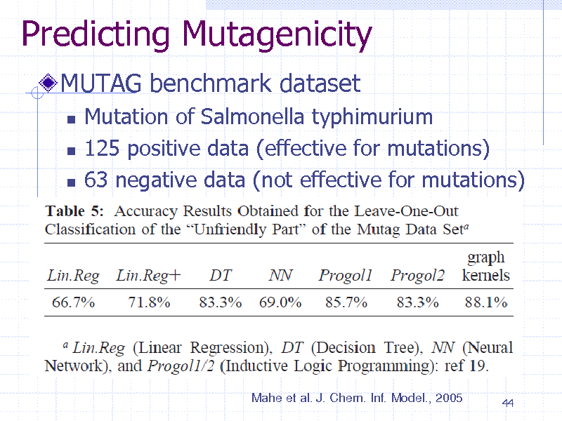
Predicting Mutagenicity
MUTAG benchmark dataset
Mutation of Salmonella typhimurium 125 positive data (effective for mutations) 63 negative data (not effective for mutations)
Mahe et al. J. Chem. Inf. Model., 2005
44
255
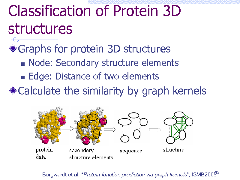
Classification of Protein 3D structures
Graphs for protein 3D structures
Node: Secondary structure elements Edge: Distance of two elements
Calculate the similarity by graph kernels
45 Borgwardt et al. Protein function prediction via graph kernels, ISMB2005
256
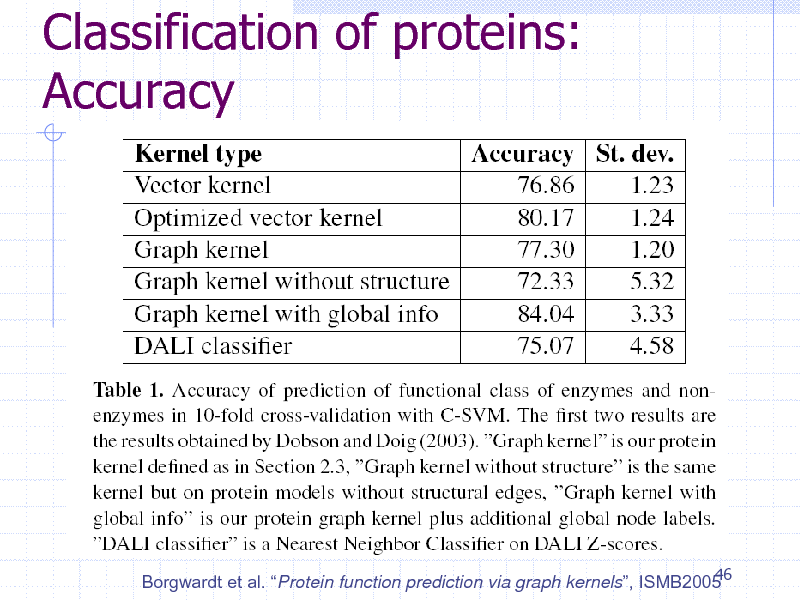
Classification of proteins: Accuracy
46 Borgwardt et al. Protein function prediction via graph kernels, ISMB2005
257
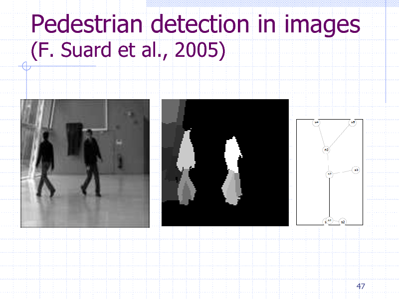
Pedestrian detection in images
(F. Suard et al., 2005)
47
258
Classifying RNA graphs
Karklin et al.,, 2005)
(Y.
48
259
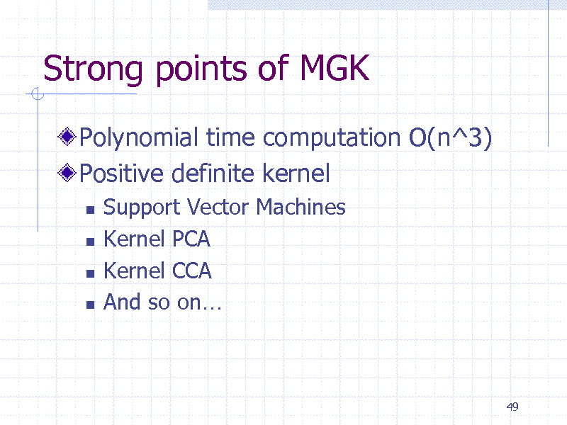
Strong points of MGK
Polynomial time computation O(n^3) Positive definite kernel
Support Vector Machines Kernel PCA Kernel CCA And so on
49
260

Drawbacks of graph kernels
Global similarity measure
Fails to capture subtle differences Long paths suppressed
Results not interpretable
Structural features ignored (e.g. loops)
No labels -> kernel always 1
50
261
Part 4. Weisfeiler Lehman kernel
51
262
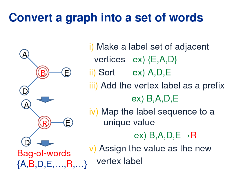
Convert a graph into a set of words
i) Make a label set of adjacent A vertices ex) {E,A,D} ii) Sort ex) A,D,E B E iii) Add the vertex label as a prefix D ex) B,A,D,E A iv) Map the label sequence to a unique value E R ex) B,A,D,ER D v) Assign the value as the new Bag-of-words {A,B,D,E,,R,} vertex label
263
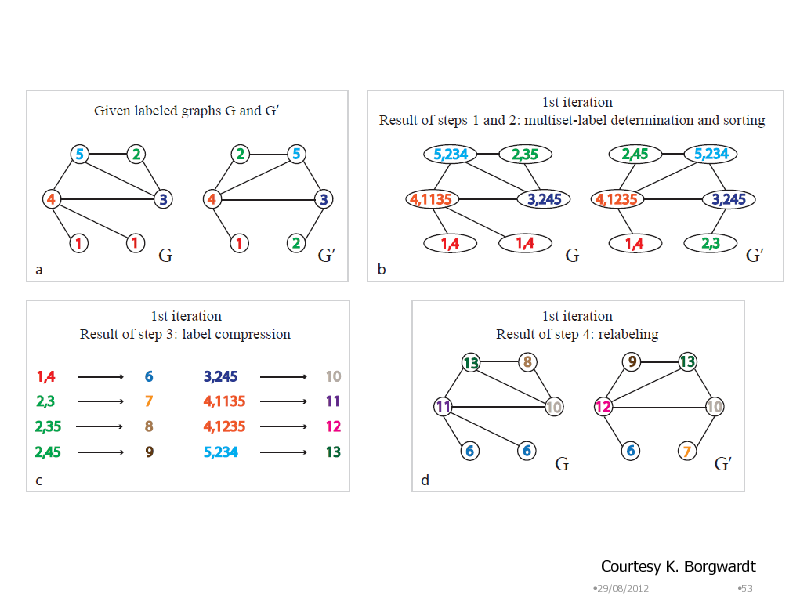
Courtesy K. Borgwardt
29/08/2012 53
264
54
265

Part 5. Reaction Graph Kernels
55
266
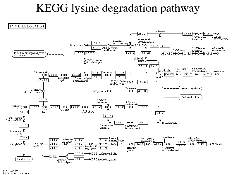
KEGG lysine degradation pathway
267
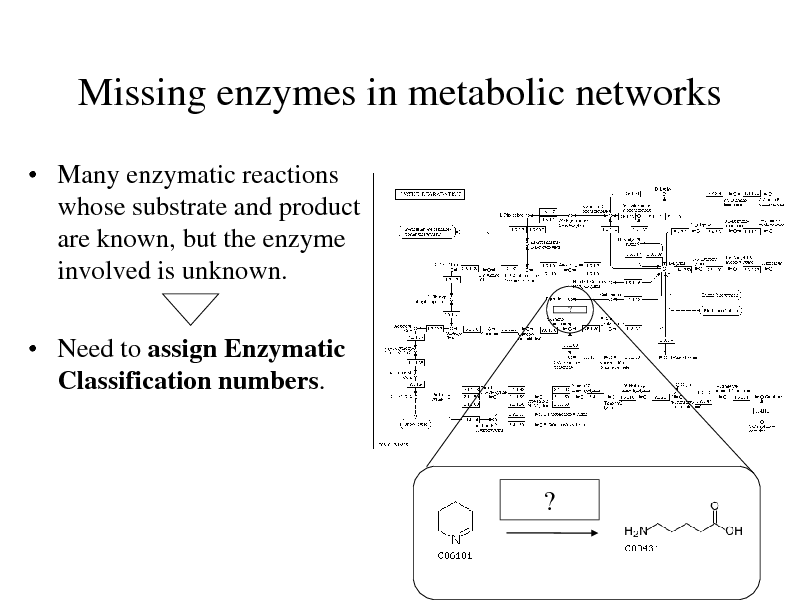
Missing enzymes in metabolic networks
Many enzymatic reactions whose substrate and product are known, but the enzyme involved is unknown.
?
Need to assign Enzymatic Classification numbers.
?
268

EC number
EC (Enzymatic Classification) number is a hierarchical categorization of
Enzymes Enzymatic reactions
class
subsubclass
EC 1.3.3.subclass
269
Task
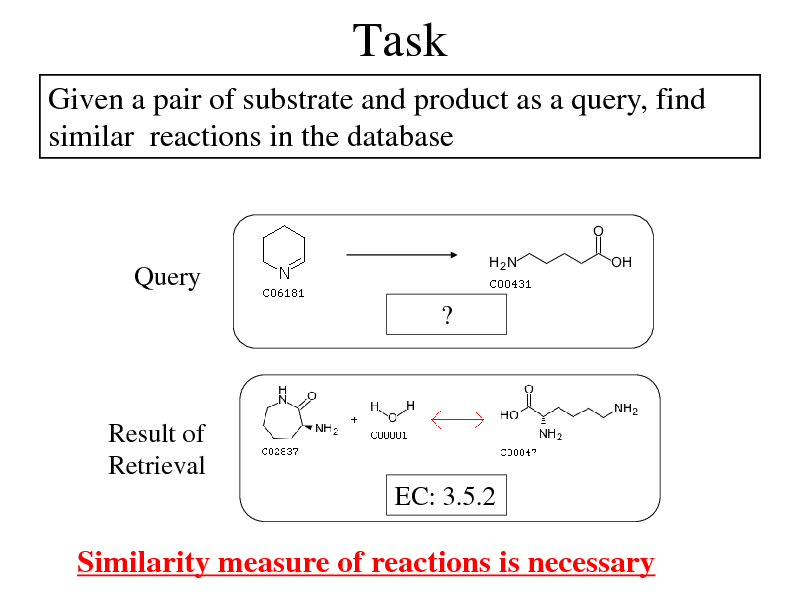
Given a pair of substrate and product as a query, find similar reactions in the database
Query ?
Result of Retrieval EC: 3.5.2
Similarity measure of reactions is necessary
270
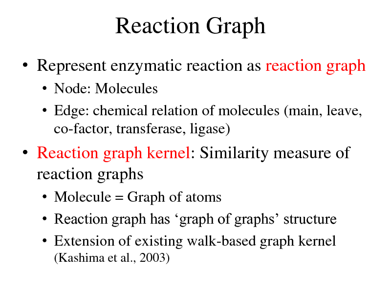
Reaction Graph
Represent enzymatic reaction as reaction graph
Node: Molecules Edge: chemical relation of molecules (main, leave, co-factor, transferase, ligase)
Reaction graph kernel: Similarity measure of reaction graphs
Molecule = Graph of atoms Reaction graph has graph of graphs structure Extension of existing walk-based graph kernel
(Kashima et al., 2003)
271
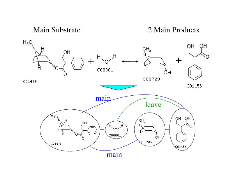
Main Substrate
2 Main Products
main
leave
main
272
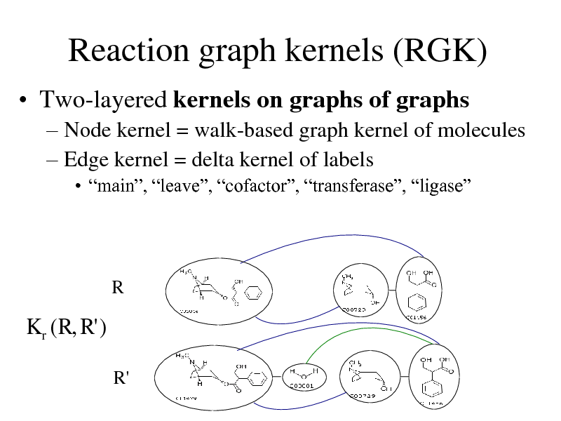
Reaction graph kernels (RGK)
Two-layered kernels on graphs of graphs
Node kernel = walk-based graph kernel of molecules Edge kernel = delta kernel of labels
main, leave, cofactor, transferase, ligase
R
K r ( R, R' )
R'
273
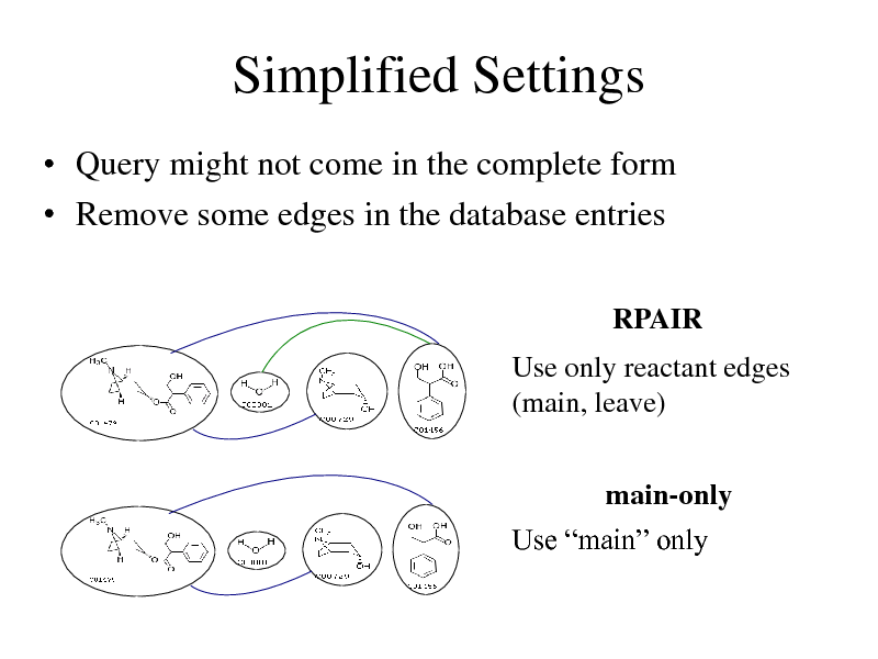
Simplified Settings
Query might not come in the complete form Remove some edges in the database entries
RPAIR
Use only reactant edges (main, leave)
main-only Use main only
274
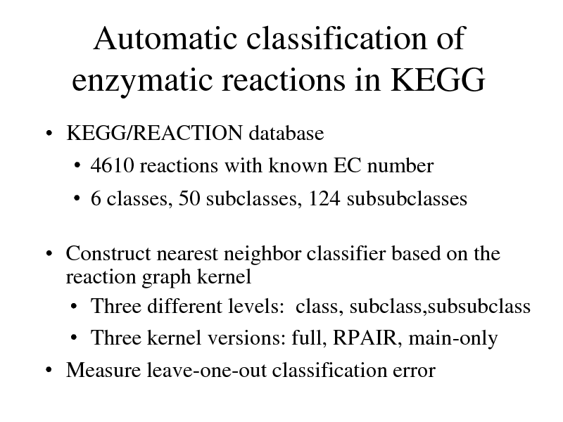
Automatic classification of enzymatic reactions in KEGG
KEGG/REACTION database 4610 reactions with known EC number 6 classes, 50 subclasses, 124 subsubclasses
Construct nearest neighbor classifier based on the reaction graph kernel Three different levels: class, subclass,subsubclass Three kernel versions: full, RPAIR, main-only Measure leave-one-out classification error
275
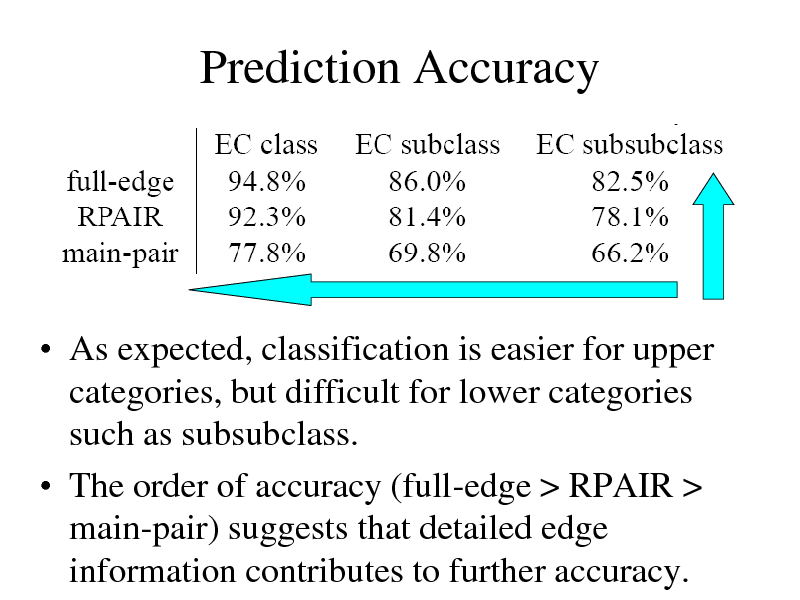
Prediction Accuracy
As expected, classification is easier for upper categories, but difficult for lower categories such as subsubclass. The order of accuracy (full-edge > RPAIR > main-pair) suggests that detailed edge information contributes to further accuracy.
276
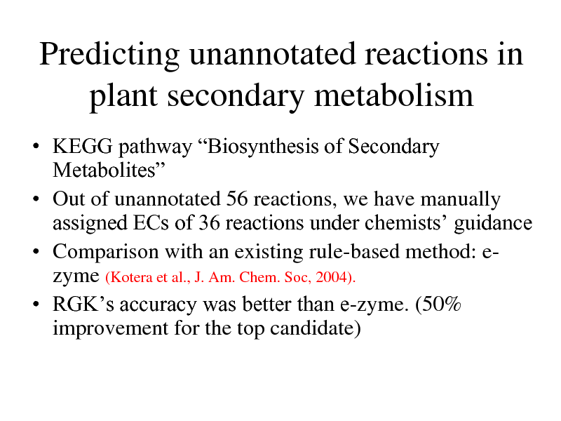
Predicting unannotated reactions in plant secondary metabolism
KEGG pathway Biosynthesis of Secondary Metabolites Out of unannotated 56 reactions, we have manually assigned ECs of 36 reactions under chemists guidance Comparison with an existing rule-based method: ezyme (Kotera et al., J. Am. Chem. Soc, 2004). RGKs accuracy was better than e-zyme. (50% improvement for the top candidate)
277
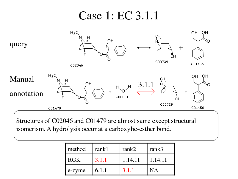
Case 1: EC 3.1.1
query
Manual
3.1.1
annotation
Structures of C02046 and C01479 are almost same except structural isomerism. A hydrolysis occur at a carboxylic-esther bond.
method RGK rank1 3.1.1 rank2 1.14.11 rank3 1.14.11
e-zyme
6.1.1
3.1.1
NA
278
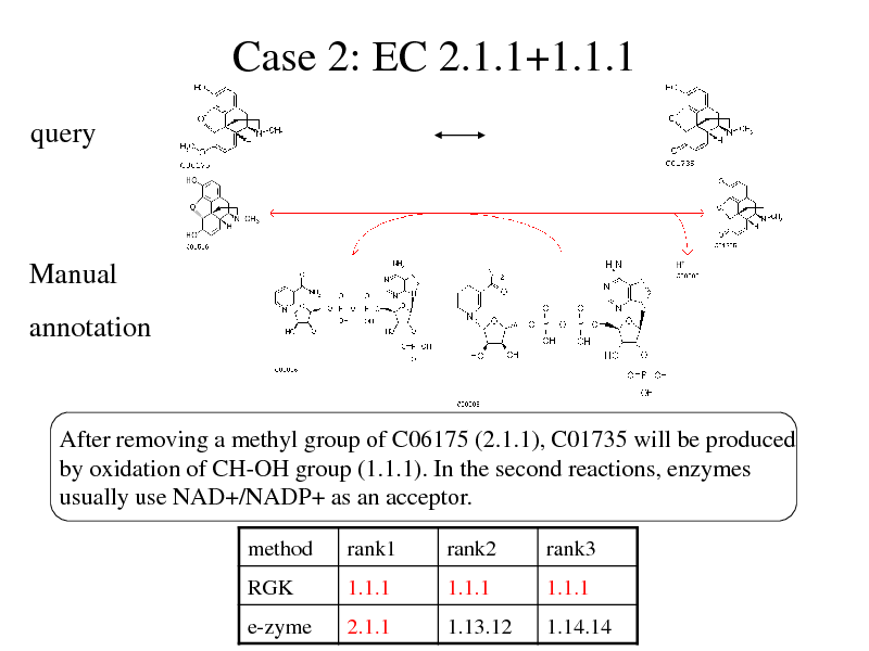
Case 2: EC 2.1.1+1.1.1
query
Manual
annotation
After removing a methyl group of C06175 (2.1.1), C01735 will be produced by oxidation of CH-OH group (1.1.1). In the second reactions, enzymes usually use NAD+/NADP+ as an acceptor.
method
RGK e-zyme
rank1
1.1.1 2.1.1
rank2
1.1.1 1.13.12
rank3
1.1.1 1.14.14
279
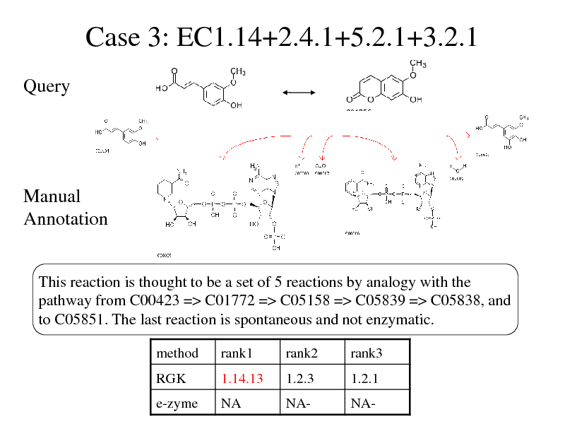
Case 3: EC1.14+2.4.1+5.2.1+3.2.1
Query
Manual Annotation
This reaction is thought to be a set of 5 reactions by analogy with the pathway from C00423 => C01772 => C05158 => C05839 => C05838, and to C05851. The last reaction is spontaneous and not enzymatic.
method RGK rank1 1.14.13 rank2 1.2.3 rank3 1.2.1
e-zyme
NA
NA-
NA-
280
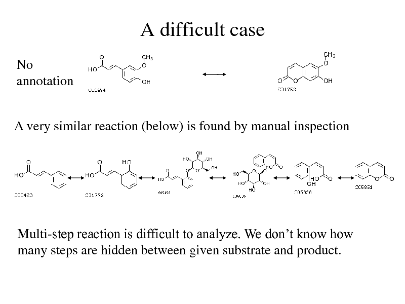
A difficult case
No annotation
A very similar reaction (below) is found by manual inspection
Multi-step reaction is difficult to analyze. We dont know how many steps are hidden between given substrate and product.
281
Concluding Remarks: New Frontier
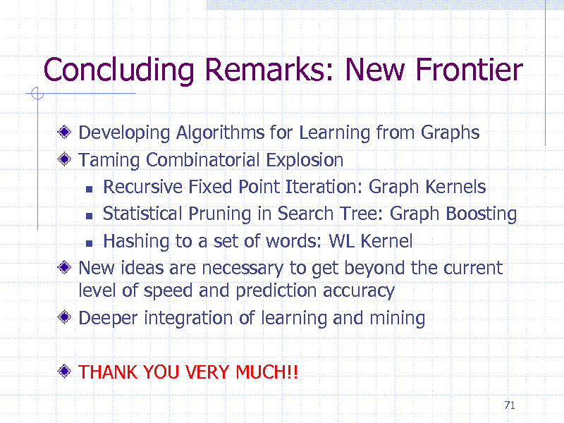
Developing Algorithms for Learning from Graphs Taming Combinatorial Explosion Recursive Fixed Point Iteration: Graph Kernels Statistical Pruning in Search Tree: Graph Boosting Hashing to a set of words: WL Kernel New ideas are necessary to get beyond the current level of speed and prediction accuracy Deeper integration of learning and mining
THANK YOU VERY MUCH!!
71
282
![Slide: Reference
[1] H. Kashima, K. Tsuda, and A. Inokuchi, Marginalized kernels between labeled graphs, ICML, pp. 321328, 2003. [2] H. Saigo, M. Hattori, H. Kashima, and K. Tsuda, Reaction graph kernels predict EC numbers of unknown enzymatic reactions in plant secondary metabolism., BMC bioinformatics, vol. 11 Suppl 1, no. Suppl 1, p. S31, Jan. 2010. [3] N. Shervashidze, P. Schweitzer, V. Leeuwen, E. Jan, K. Mehlhorn, and K. Borgwardt, Weisfeiler-Lehman graph kernels, Journal of Machine Learning Research, vol. 12, pp. 25392561, 2011. [4] K. Tsuda, T. Kin, and K. Asai, Marginalized kernels for biological sequences, Bioinformatics, vol. 18, no. Suppl 1, pp. S268S275, Jul. 2002.
72](https://yosinski.com/mlss12/media/slides/MLSS-2012-Tsuda-Graph-Mining_283.png)
Reference
[1] H. Kashima, K. Tsuda, and A. Inokuchi, Marginalized kernels between labeled graphs, ICML, pp. 321328, 2003. [2] H. Saigo, M. Hattori, H. Kashima, and K. Tsuda, Reaction graph kernels predict EC numbers of unknown enzymatic reactions in plant secondary metabolism., BMC bioinformatics, vol. 11 Suppl 1, no. Suppl 1, p. S31, Jan. 2010. [3] N. Shervashidze, P. Schweitzer, V. Leeuwen, E. Jan, K. Mehlhorn, and K. Borgwardt, Weisfeiler-Lehman graph kernels, Journal of Machine Learning Research, vol. 12, pp. 25392561, 2011. [4] K. Tsuda, T. Kin, and K. Asai, Marginalized kernels for biological sequences, Bioinformatics, vol. 18, no. Suppl 1, pp. S268S275, Jul. 2002.
72
283