
High-Dimensional Sampling Algorithms
Santosh Vempala
Algorithms and Randomness Center Georgia Tech
We study the complexity, in high dimension, of basic algorithmic problems such as optimization, integration, rounding and sampling. A suitable convexity assumption allows polynomial-time algorithms for these problems, while still including very interesting special cases such as linear programming, volume computation and many instances of discrete optimization. We will survey the breakthroughs that lead to the current state-of-the-art and pay special attention to the discovery that all of the above problems can be reduced to the problem of *sampling* efficiently. In the process of establishing upper and lower bounds on the complexity of sampling in high dimension, we will encounter geometric random walks, isoperimetric inequalities, generalizations of convexity, probabilistic proof techniques and other methods bridging geometry, probability and complexity.
Scroll with j/k | | | Size

High-Dimensional Sampling Algorithms
Santosh Vempala
Algorithms and Randomness Center Georgia Tech
1

Format
Please ask questions Indicate that I should go faster or slower Feel free to ask for more examples And for more proofs
Exercises along the way.
2
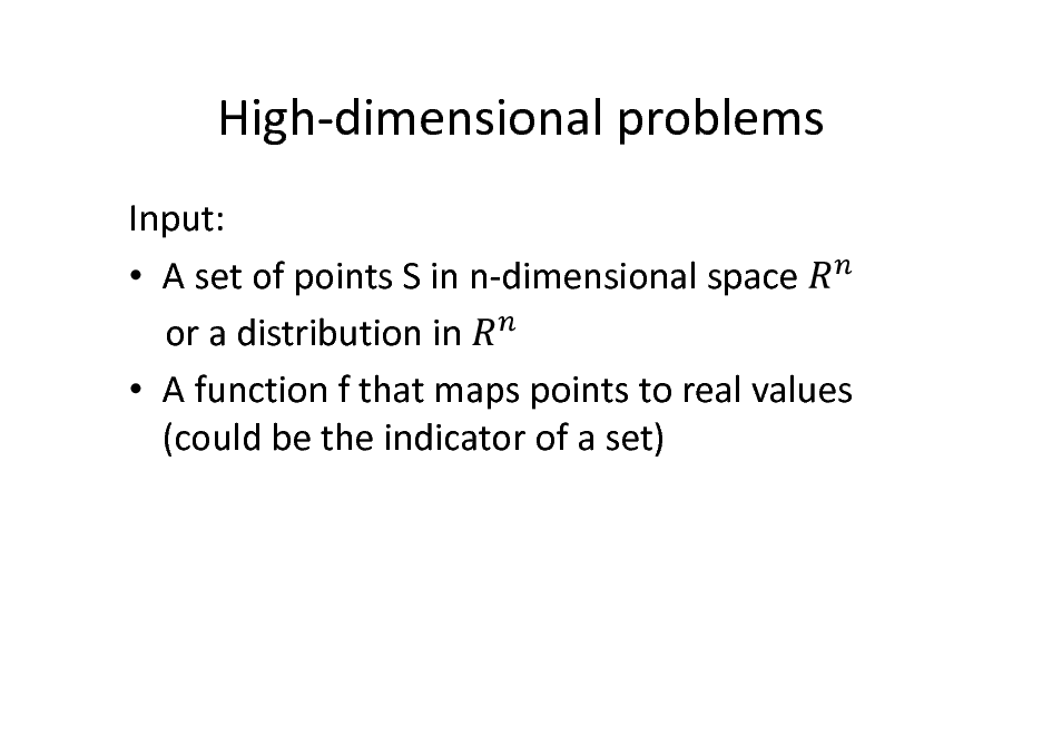
High-dimensional problems
Input: A set of points S in n-dimensional space or a distribution in A function f that maps points to real values (could be the indicator of a set)
3

Algorithmic Geometry
What is the complexity of computational problems as the dimension grows? Dimension = number of variables
Typically, size of input is a function of the dimension.
4
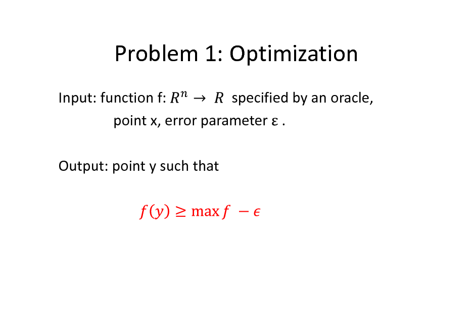
Problem 1: Optimization
Input: function f: specified by an oracle, point x, error parameter . Output: point y such that
5
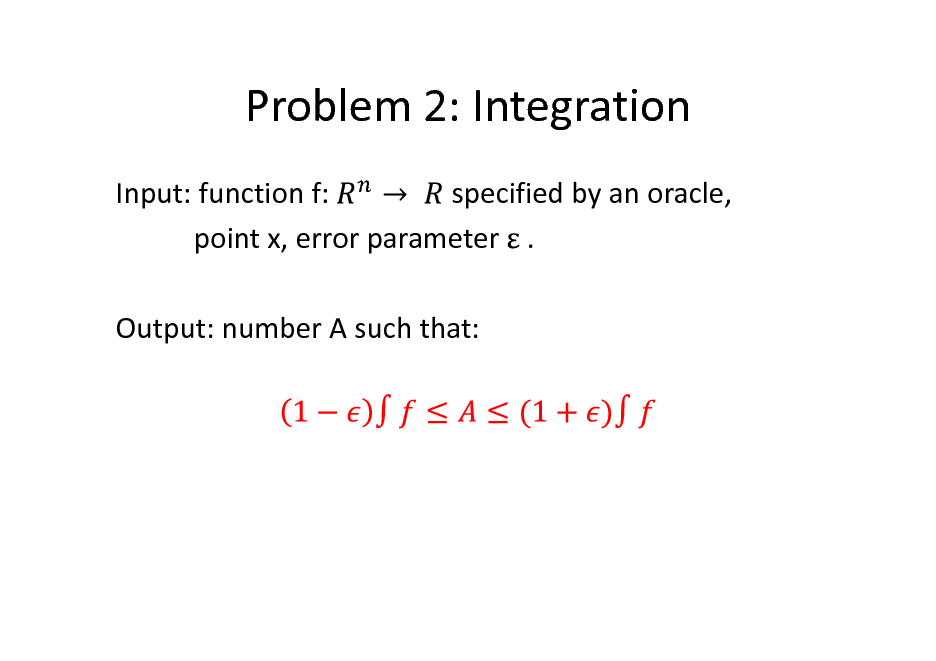
Problem 2: Integration
Input: function f: specified by an oracle, point x, error parameter . Output: number A such that:
6
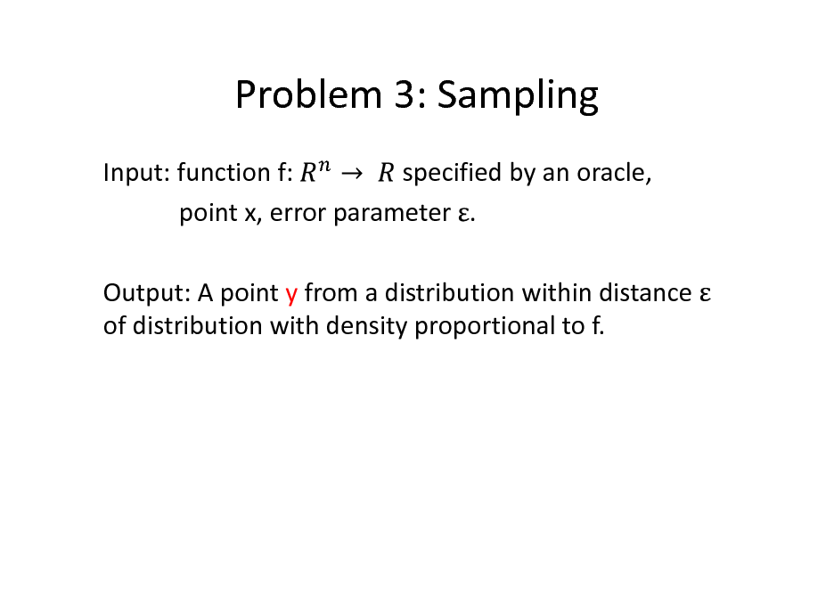
Problem 3: Sampling
Input: function f: specified by an oracle, point x, error parameter . Output: A point y from a distribution within distance of distribution with density proportional to f.
7
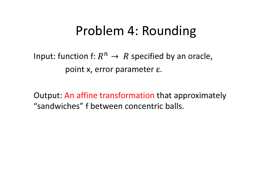
Problem 4: Rounding
Input: function f: specified by an oracle, point x, error parameter . Output: An affine transformation that approximately sandwiches f between concentric balls.
8
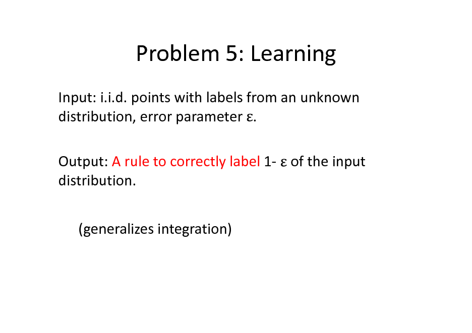
Problem 5: Learning
Input: i.i.d. points with labels from an unknown distribution, error parameter . Output: A rule to correctly label 1- of the input distribution. (generalizes integration)
9

Sampling
Generate a uniform random point from a set S or with density proportional to function f. Numerous applications in diverse areas: statistics, networking, biology, computer vision, privacy, operations research etc. This course: mathematical and algorithmic foundations of sampling and its applications.
10
Course Outline
Lecture 1. Introduction to Sampling, highdimensional Geometry and Complexity. L2. Algorithms based on Sampling. L3. Sampling Algorithms.
11
Lecture 1: Introduction
Computational problems in high dimension The challenges of high dimensionality Convex bodies, Logconcave functions Brunn-Minkowski and its variants Isotropy Summary of applications
12
Lecture 2: Algorithmic Applications
Convex Optimization Rounding Volume Computation Integration
13
Lecture 3: Sampling Algorithms
Sampling by random walks Conductance Grid walk, Ball walk, Hit-and-run Isoperimetric inequalities Rapid mixing
14

High-dimensional problems are hard
P1. Optimization. Find minimum of f over a set. P2. Integration. Find the average (or integral) of f. These problems are intractable (hard) in general, i.e., for arbitrary sets and general functions Intractable for arbitrary sets and linear functions Intractable for polytopes and quadratic functions P1 is NP-hard or worse
min number of unsatisfied clauses in a 3-SAT formula
P2 is #P-hard or worse
Count number of satisfying solutions to a 3-SAT formula
15
![Slide: High-dimensional Algorithms
P1. Optimization. Find minimum of f over the set S. Ellipsoid algorithm [Yudin-Nemirovski; Shor;Khachiyan;GLS] S is a convex set and f is a convex function. P2. Integration. Find the integral of f. Dyer-Frieze-Kannan algorithm f is the indicator function of a convex set.](https://yosinski.com/mlss12/media/slides/MLSS-2012-Vempala-High-Dimensional-Sampling-Algorithms_016.png)
High-dimensional Algorithms
P1. Optimization. Find minimum of f over the set S. Ellipsoid algorithm [Yudin-Nemirovski; Shor;Khachiyan;GLS] S is a convex set and f is a convex function. P2. Integration. Find the integral of f. Dyer-Frieze-Kannan algorithm f is the indicator function of a convex set.
16
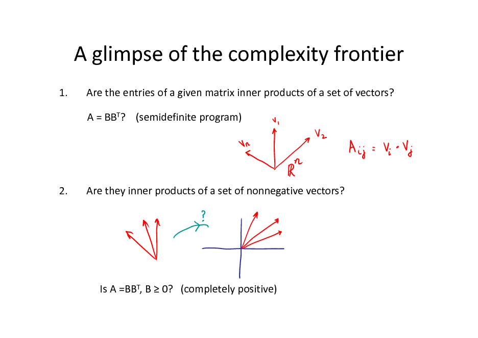
A glimpse of the complexity frontier
1. Are the entries of a given matrix inner products of a set of vectors? A = BBT? (semidefinite program)
2.
Are they inner products of a set of nonnegative vectors?
Is A =BBT, B 0? (completely positive)
17

Structure
Q. What geometric structure makes algorithmic problems computationally tractable?
(i.e., solvable with polynomial complexity)
Convexity often suffices. Is convexity the frontier of polynomial-time solvability? Appears to be in many cases of interest
18
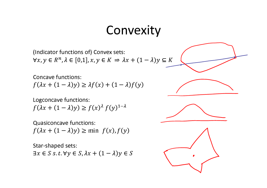
Convexity
(Indicator functions of) Convex sets: , , 0,1 , , + 1 Concave functions: + 1 Logconcave functions: + 1 Quasiconcave functions: + 1 min Star-shaped sets: . . , + 1 ,
+ 1
19
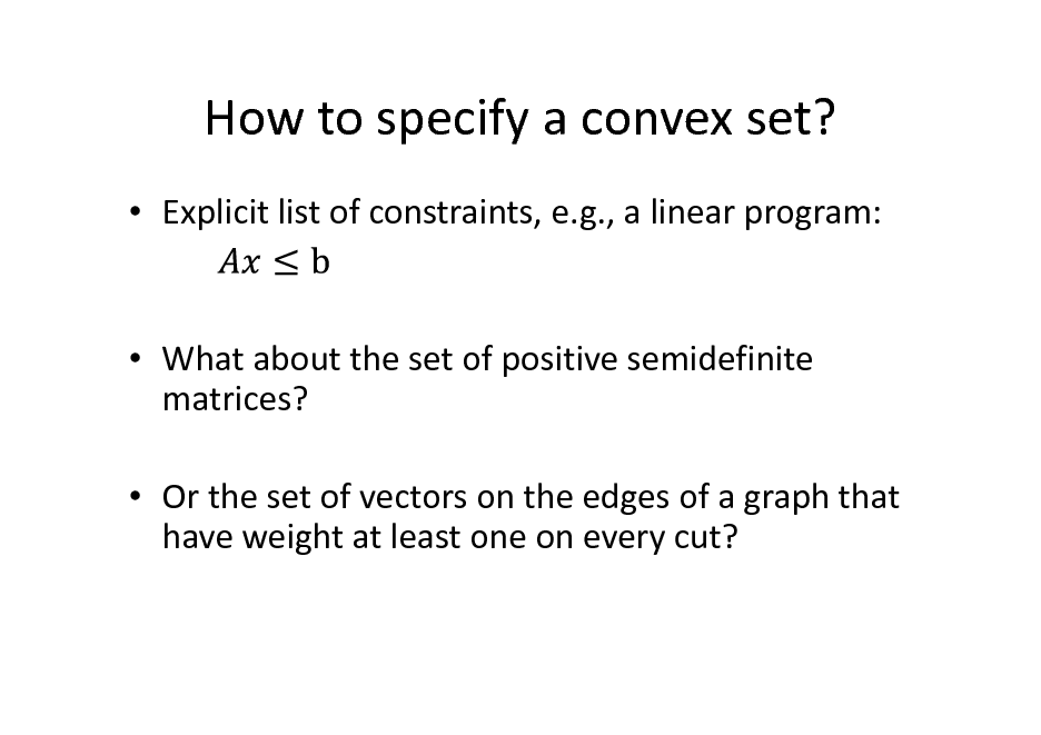
How to specify a convex set?
Explicit list of constraints, e.g., a linear program:
What about the set of positive semidefinite matrices? Or the set of vectors on the edges of a graph that have weight at least one on every cut?
20
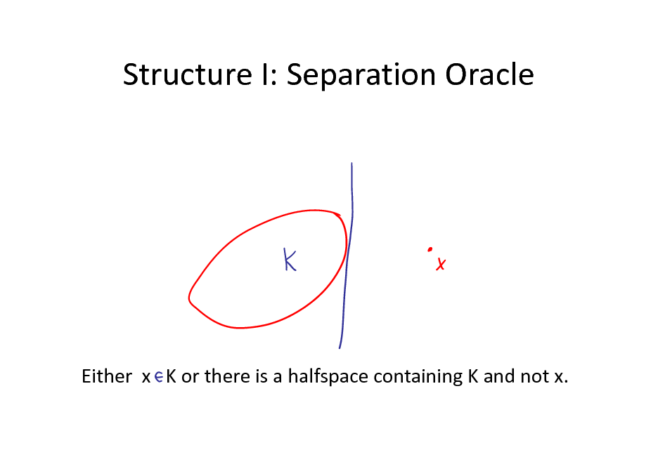
Structure I: Separation Oracle
Either x K or there is a halfspace containing K and not x.
21
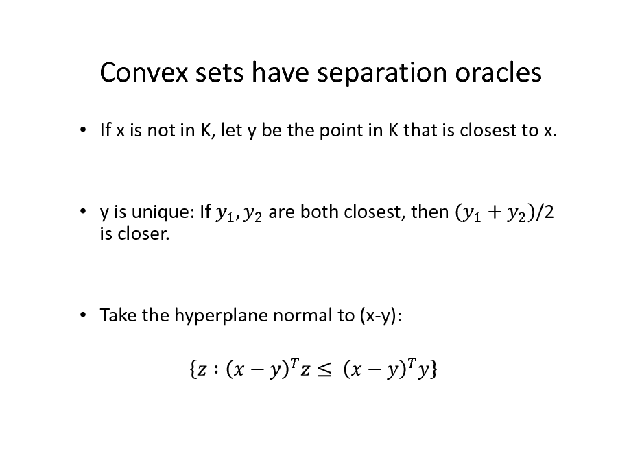
Convex sets have separation oracles
If x is not in K, let y be the point in K that is closest to x.
y is unique: If is closer.
are both closest, then
/2
Take the hyperplane normal to (x-y):
22
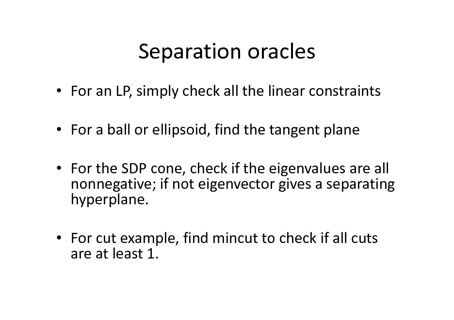
Separation oracles
For an LP, simply check all the linear constraints For a ball or ellipsoid, find the tangent plane For the SDP cone, check if the eigenvalues are all nonnegative; if not eigenvector gives a separating hyperplane. For cut example, find mincut to check if all cuts are at least 1.
23
Example: Learning by Sampling
Sequence of points X1, X2, , Unknown -1/1 function f We get Xi and have to guess f(Xi) Goal: minimize number of wrong guesses.
24
Learning Halfspaces
Unknown -1/1 function f f(X) = 1 if > 0 and f(X) = -1 otherwise
For an unknown vector w, with each component wi being a b-bit integer. What is the minimum number of mistakes?
25
Majority algorithm
After X1, X2, ,Xk the set of consistent functions f correspond to Sk = {w : (sign(Xi)Xi) > 0 for i = 1,2,, k } Guess f(Xk+1), to be the majority of the predictions of each w in Sk Claim. Number of wrong guesses bn But how to compute majority?? |Sk| could be 2bn !
26
Random algorithm
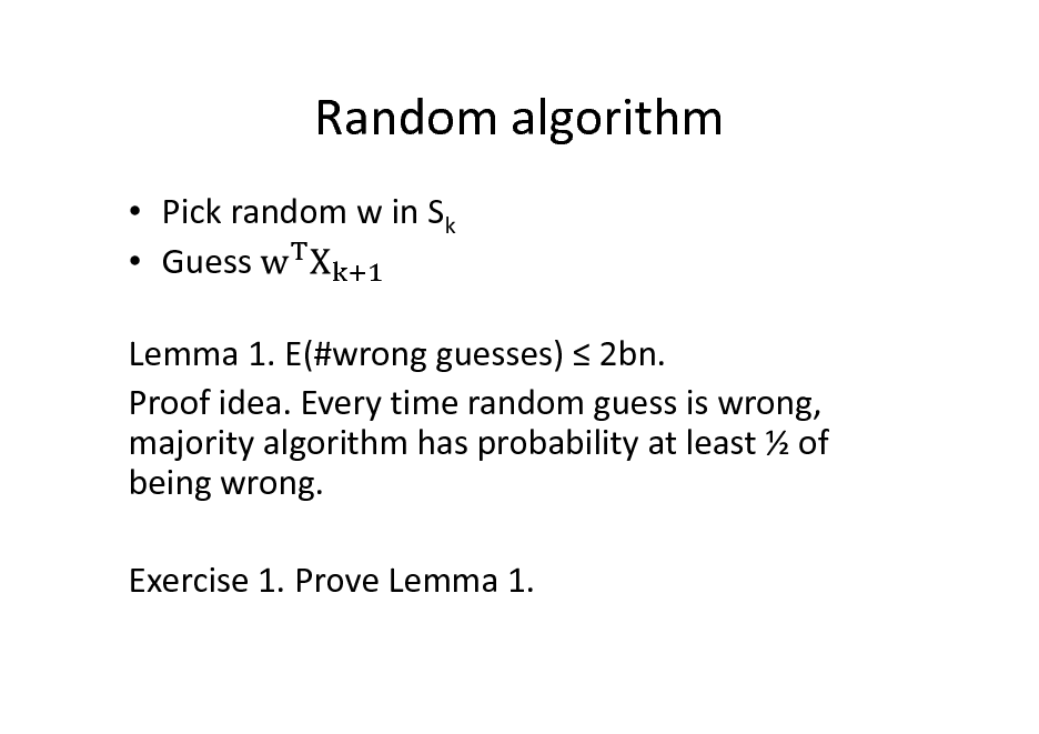
Pick random w in Sk Guess
27
Random algorithm
Pick random w in Sk Guess Lemma 1. E(#wrong guesses) 2bn. Proof idea. Every time random guess is wrong, majority algorithm has probability at least of being wrong. Exercise 1. Prove Lemma 1.
28
Learning by Sampling
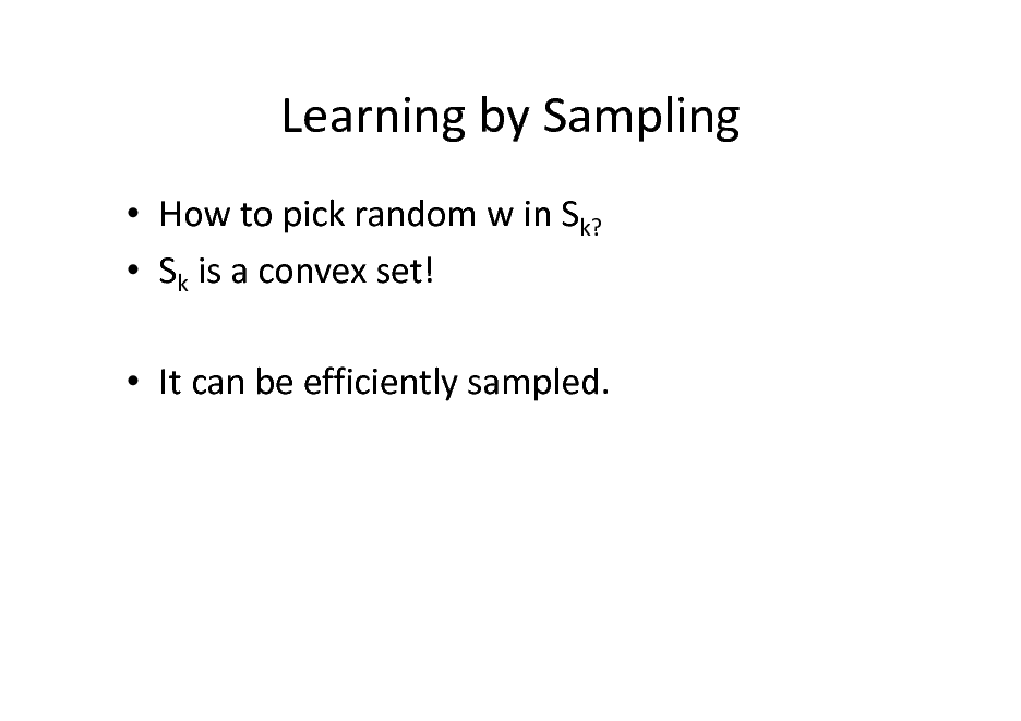
How to pick random w in Sk? Sk is a convex set! It can be efficiently sampled.
29
Structure of Convex Bodies
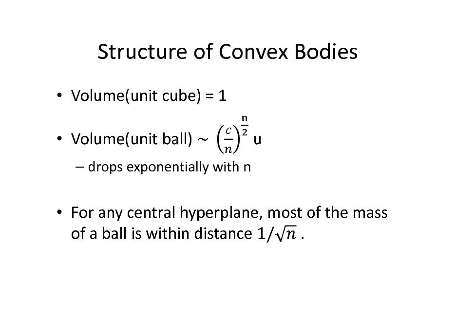
Volume(unit cube) = 1 Volume(unit ball)
drops exponentially with n
u
For any central hyperplane, most of the mass . of a ball is within distance
30
Structure of Convex Bodies
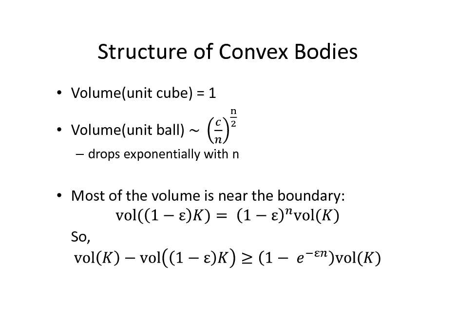
Volume(unit cube) = 1 Volume(unit ball)
drops exponentially with n
Most of the volume is near the boundary: So,
31
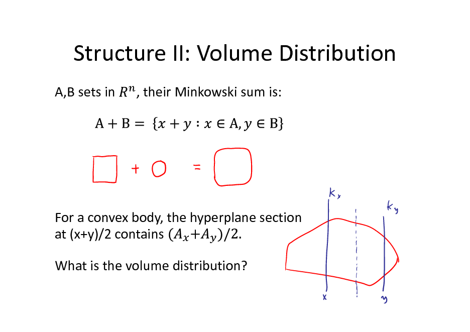
Structure II: Volume Distribution
A,B sets in , their Minkowski sum is:
For a convex body, the hyperplane section at (x+y)/2 contains What is the volume distribution?
32
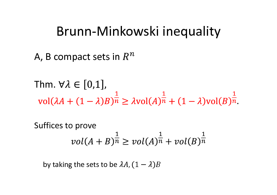
Brunn-Minkowski inequality
A, B compact sets in Thm.
Suffices to prove
by taking the sets to be
, 1
33
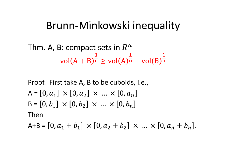
Brunn-Minkowski inequality
Thm. A, B: compact sets in
Proof. First take A, B to be cuboids, i.e., A= B= Then A+B =
.
34
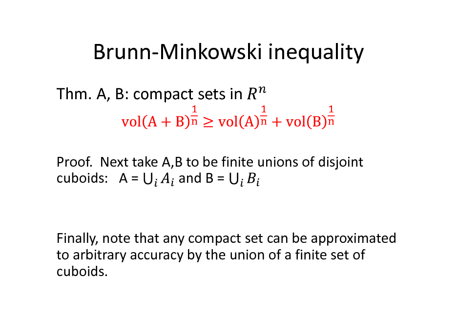
Brunn-Minkowski inequality
Thm. A, B: compact sets in
Proof. Next take A,B to be finite unions of disjoint cuboids: A = and B =
Finally, note that any compact set can be approximated to arbitrary accuracy by the union of a finite set of cuboids.
35
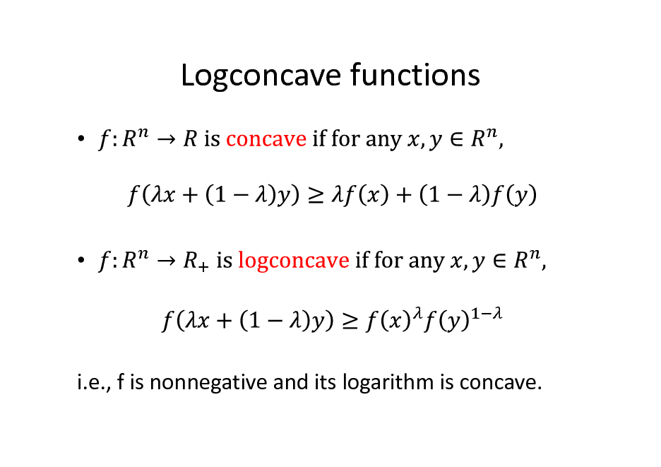
Logconcave functions
i.e., f is nonnegative and its logarithm is concave.
36
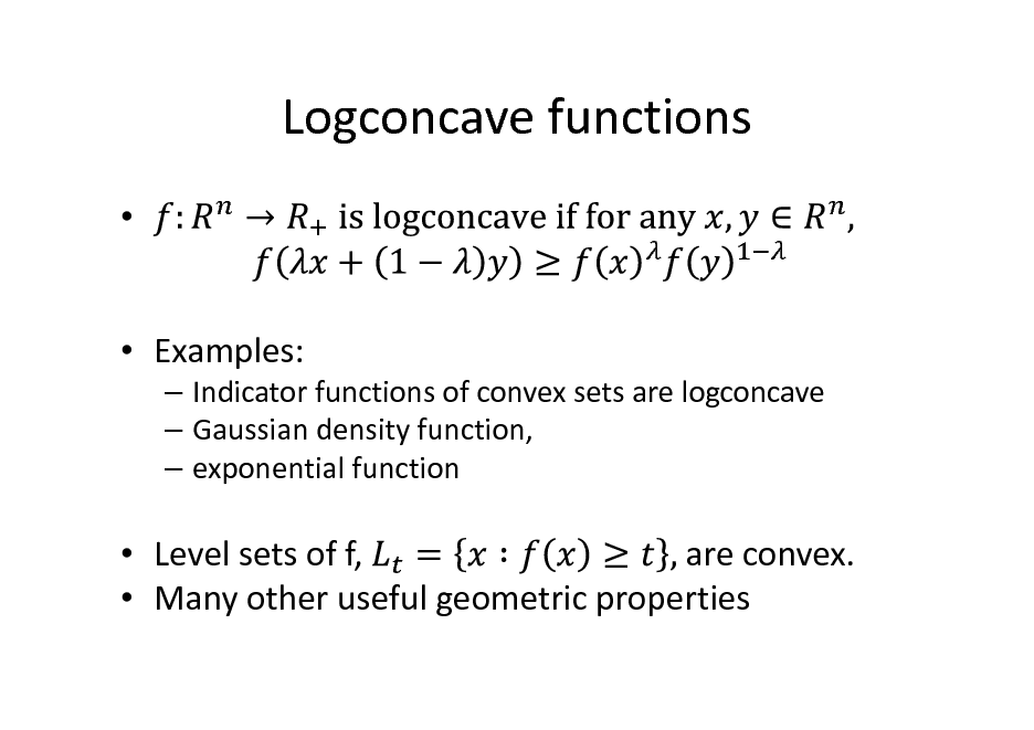
Logconcave functions
Examples:
Indicator functions of convex sets are logconcave Gaussian density function, exponential function
Level sets of f, are convex. Many other useful geometric properties
37
![Slide: Prekopa-Leindler inequality
Prekopa-Leindler: then
Functional version of [B-M], equivalent to it.](https://yosinski.com/mlss12/media/slides/MLSS-2012-Vempala-High-Dimensional-Sampling-Algorithms_038.png)
Prekopa-Leindler inequality
Prekopa-Leindler: then
Functional version of [B-M], equivalent to it.
38
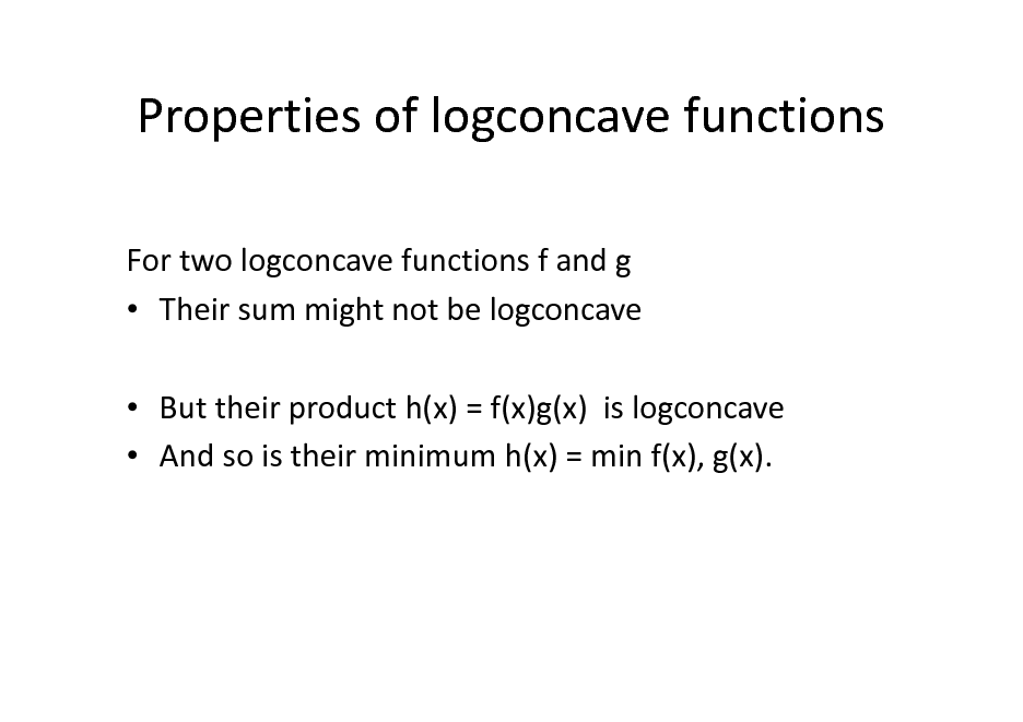
Properties of logconcave functions
For two logconcave functions f and g Their sum might not be logconcave But their product h(x) = f(x)g(x) is logconcave And so is their minimum h(x) = min f(x), g(x).
39
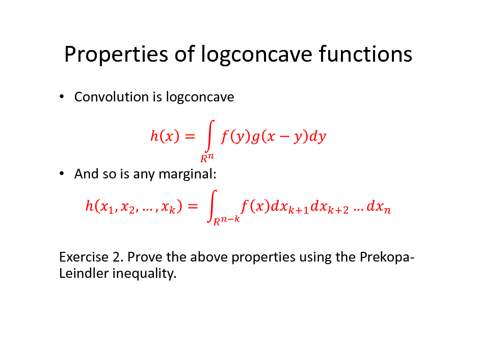
Properties of logconcave functions
Convolution is logconcave
And so is any marginal:
Exercise 2. Prove the above properties using the PrekopaLeindler inequality.
40
Isotropic position
Affine transformations preserve convexity and logconcavity. What can one use as a canonical position? E.g., ellipsoids map to a ball, parallelopipeds map to cubes. What about general convex bodies? Logconcave functions?
41
Isotropic position
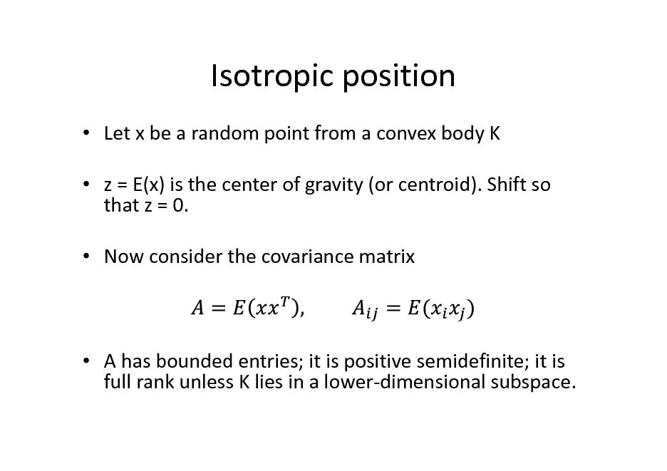
Let x be a random point from a convex body K z = E(x) is the center of gravity (or centroid). Shift so that z = 0. Now consider the covariance matrix
A has bounded entries; it is positive semidefinite; it is full rank unless K lies in a lower-dimensional subspace.
42
Isotropic position
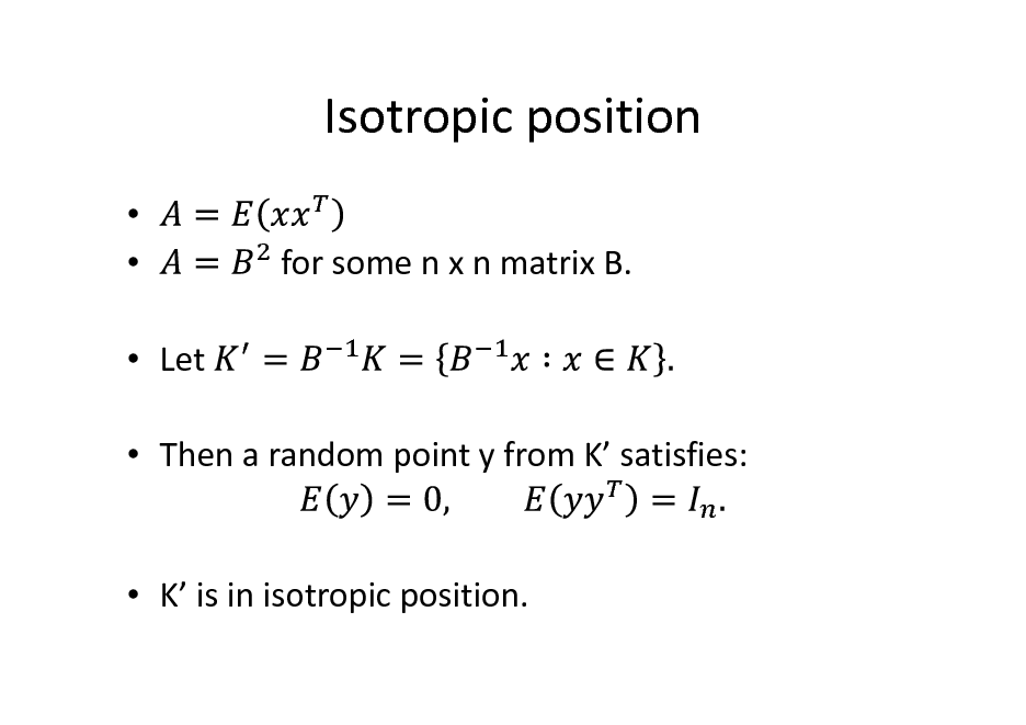
Let Then a random point y from K satisfies: for some n x n matrix B.
K is in isotropic position.
43
Isotropic position: Exercises
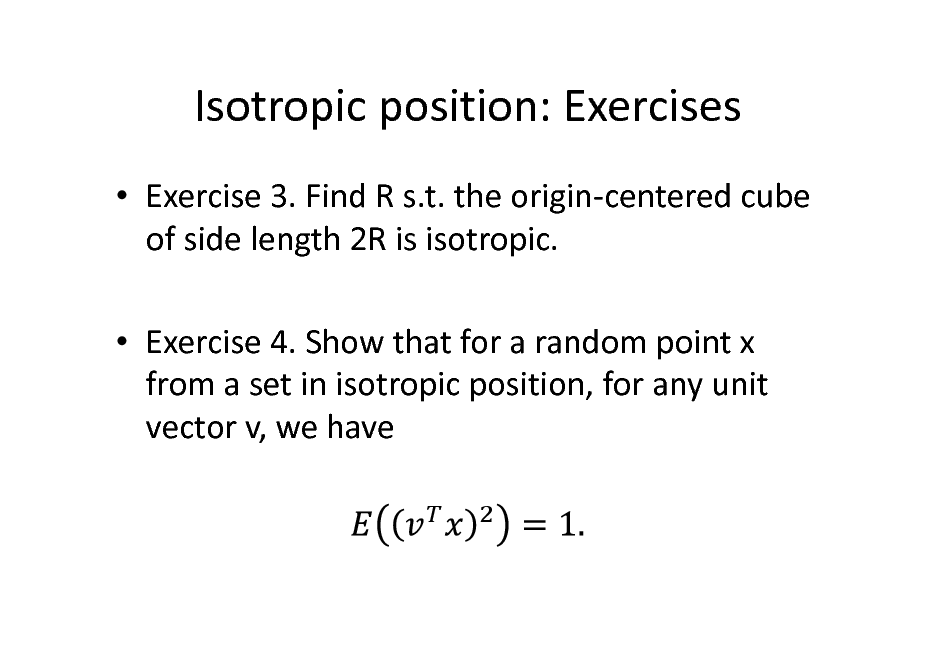
Exercise 3. Find R s.t. the origin-centered cube of side length 2R is isotropic. Exercise 4. Show that for a random point x from a set in isotropic position, for any unit vector v, we have
44
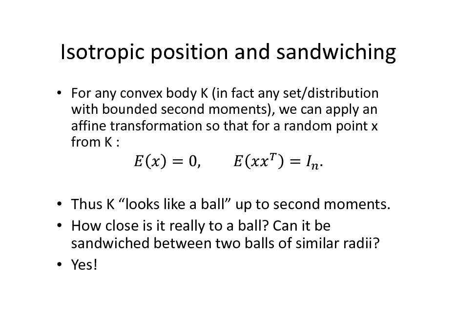
Isotropic position and sandwiching
For any convex body K (in fact any set/distribution with bounded second moments), we can apply an affine transformation so that for a random point x from K :
Thus K looks like a ball up to second moments. How close is it really to a ball? Can it be sandwiched between two balls of similar radii? Yes!
45
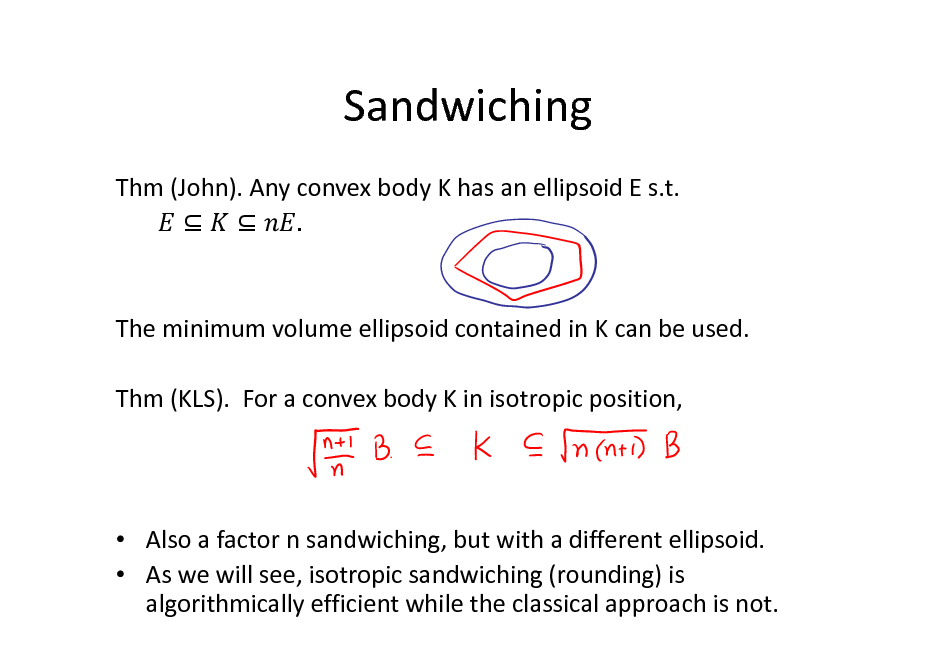
Sandwiching
Thm (John). Any convex body K has an ellipsoid E s.t. .
The minimum volume ellipsoid contained in K can be used. Thm (KLS). For a convex body K in isotropic position,
Also a factor n sandwiching, but with a different ellipsoid. As we will see, isotropic sandwiching (rounding) is algorithmically efficient while the classical approach is not.
46

Lecture 2: Algorithmic Applications
Convex Optimization Rounding Volume Computation Integration
47

Lecture 3: Sampling Algorithms
Sampling by random walks Conductance Grid walk, Ball walk, Hit-and-run Isoperimetric inequalities Rapid mixing
48

High-Dimensional Sampling Algorithms
Santosh Vempala
Algorithms and Randomness Center Georgia Tech
49
Format
Please ask questions Indicate that I should go faster or slower Feel free to ask for more examples And for more proofs
Exercises along the way.
50
High-dimensional problems
Input: or a distribution in A set of points S in A function f that maps points to real values (could be the indicator of a set)
51
Algorithmic Geometry
What is the complexity of computational problems as the dimension grows? Dimension = number of variables
Typically, size of input is a function of the dimension.
52

Problem 1: Optimization
Input: function f: specified by an oracle, point x, error parameter . Output: point y such that
53

Problem 2: Integration
Input: function f: specified by an oracle, point x, error parameter . Output: number A such that:
54

Problem 3: Sampling
Input: function f: specified by an oracle, point x, error parameter . Output: A point y from a distribution within distance of distribution with density proportional to f.
55

Problem 4: Rounding
Input: function f: specified by an oracle, point x, error parameter . Output: An affine transformation that approximately sandwiches f between concentric balls.
56
Problem 5: Learning
Input: i.i.d. points (with labels) from unknown distribution, error parameter . Output: A rule to correctly label 1- of the input distribution. (generalizes integration)
57

Sampling
Generate a uniform random point from a set S or with density proportional to function f. Numerous applications in diverse areas: statistics, networking, biology, computer vision, privacy, operations research etc. This course: mathematical and algorithmic foundations of sampling and its applications.
58
Lecture 2: Algorithmic Applications
Given a blackbox for sampling, we will study algorithms for: Rounding Convex Optimization Volume Computation Integration
59
![Slide: High-dimensional Algorithms
P1. Optimization. Find minimum of f over the set S. Ellipsoid algorithm [Yudin-Nemirovski; Shor] works when S is a convex set and f is a convex function. P2. Integration. Find the integral of f. Dyer-Frieze-Kannan algorithm works when f is the indicator function of a convex set.](https://yosinski.com/mlss12/media/slides/MLSS-2012-Vempala-High-Dimensional-Sampling-Algorithms_060.png)
High-dimensional Algorithms
P1. Optimization. Find minimum of f over the set S. Ellipsoid algorithm [Yudin-Nemirovski; Shor] works when S is a convex set and f is a convex function. P2. Integration. Find the integral of f. Dyer-Frieze-Kannan algorithm works when f is the indicator function of a convex set.
60

Structure
Q. What geometric structure makes algorithmic problems computationally tractable?
(i.e., solvable with polynomial complexity)
Convexity often suffices. Is convexity the frontier of polynomial-time solvability? Appears to be in many cases of interest
61

Convexity
(Indicator functions of) Convex sets: , , 0,1 , , + 1 Concave functions: + 1 Logconcave functions: + 1 Quasiconcave functions: + 1 min Star-shaped sets: . . , + 1 ,
+ 1
62

Sandwiching
Thm (John). Any convex body K has an ellipsoid E s.t. .
The minimum volume ellipsoid contained in K can be used. Thm (KLS). For a convex body K in isotropic position,
Also a factor n sandwiching, but with a different ellipsoid. As we will see, isotropic sandwiching (rounding) is algorithmically efficient while the classical approach is not.
63
![Slide: Rounding via Sampling
1. Sample m random points from K; 2. Compute sample mean z and sample covariance matrix A. 3. Compute B = A . Applying B to K achieves near-isotropic position. Thm. C().n random points suffice to achieve for isotropic K.
[Adamczak et al.;Srivastava-Vershynin; improving on Bourgain;Rudelson]
I.e., for any unit vector v,
1+
1+ .](https://yosinski.com/mlss12/media/slides/MLSS-2012-Vempala-High-Dimensional-Sampling-Algorithms_064.png)
Rounding via Sampling
1. Sample m random points from K; 2. Compute sample mean z and sample covariance matrix A. 3. Compute B = A . Applying B to K achieves near-isotropic position. Thm. C().n random points suffice to achieve for isotropic K.
[Adamczak et al.;Srivastava-Vershynin; improving on Bourgain;Rudelson]
I.e., for any unit vector v,
1+
1+ .
64
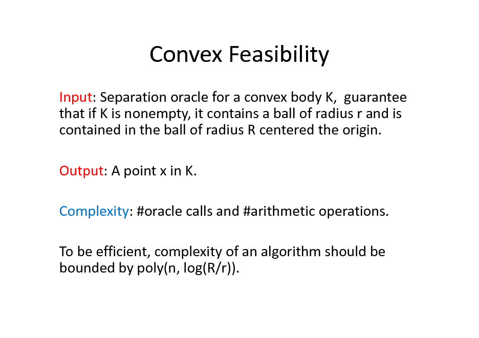
Convex Feasibility
Input: Separation oracle for a convex body K, guarantee that if K is nonempty, it contains a ball of radius r and is contained in the ball of radius R centered the origin. Output: A point x in K. Complexity: #oracle calls and #arithmetic operations. To be efficient, complexity of an algorithm should be bounded by poly(n, log(R/r)).
65
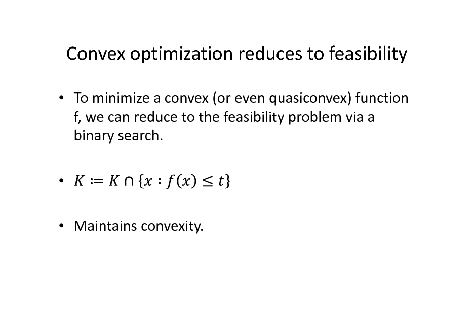
Convex optimization reduces to feasibility
To minimize a convex (or even quasiconvex) function f, we can reduce to the feasibility problem via a binary search. Maintains convexity.
66
How to choose oracle queries?
67
![Slide: Convex feasibility via sampling
[Bertsimas-V. 02] . 1. Let z=0, P = 2. Does If yes, output K. be a halfspace 3. If no, let H = containing K. 4. Let 5. Sample uniformly from P. 6. Let Go to Step 2.](https://yosinski.com/mlss12/media/slides/MLSS-2012-Vempala-High-Dimensional-Sampling-Algorithms_068.png)
Convex feasibility via sampling
[Bertsimas-V. 02] . 1. Let z=0, P = 2. Does If yes, output K. be a halfspace 3. If no, let H = containing K. 4. Let 5. Sample uniformly from P. 6. Let Go to Step 2.
68
![Slide: Centroid algorithm
[Levin 65]. Use centroid of surviving set as query point in each iteration. #iterations = O(nlog(R/r)). Best possible. Problem: how to find centroid? #P-hard! [Rademacher 2007]](https://yosinski.com/mlss12/media/slides/MLSS-2012-Vempala-High-Dimensional-Sampling-Algorithms_069.png)
Centroid algorithm
[Levin 65]. Use centroid of surviving set as query point in each iteration. #iterations = O(nlog(R/r)). Best possible. Problem: how to find centroid? #P-hard! [Rademacher 2007]
69
![Slide: Why does centroid work?
Does not cut volume in half. But it does cut by a constant fraction. Thm [Grunbaum 60]. For any halfspace H containing the centroid of a convex body K,](https://yosinski.com/mlss12/media/slides/MLSS-2012-Vempala-High-Dimensional-Sampling-Algorithms_070.png)
Why does centroid work?
Does not cut volume in half. But it does cut by a constant fraction. Thm [Grunbaum 60]. For any halfspace H containing the centroid of a convex body K,
70
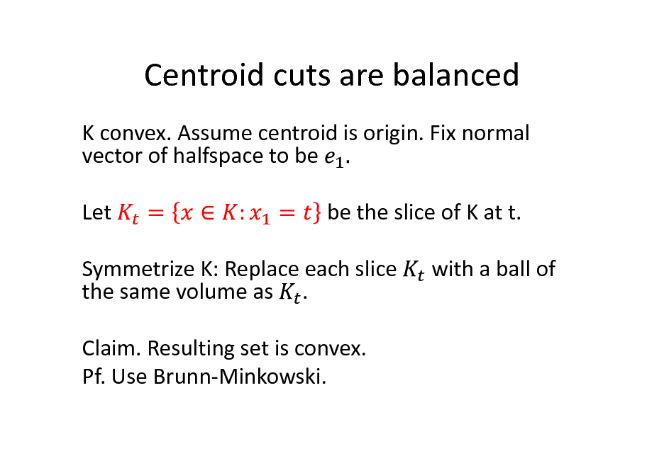
Centroid cuts are balanced
K convex. Assume centroid is origin. Fix normal vector of halfspace to be Let be the slice of K at t. with a ball of
Symmetrize K: Replace each slice the same volume as . Claim. Resulting set is convex. Pf. Use Brunn-Minkowski.
71
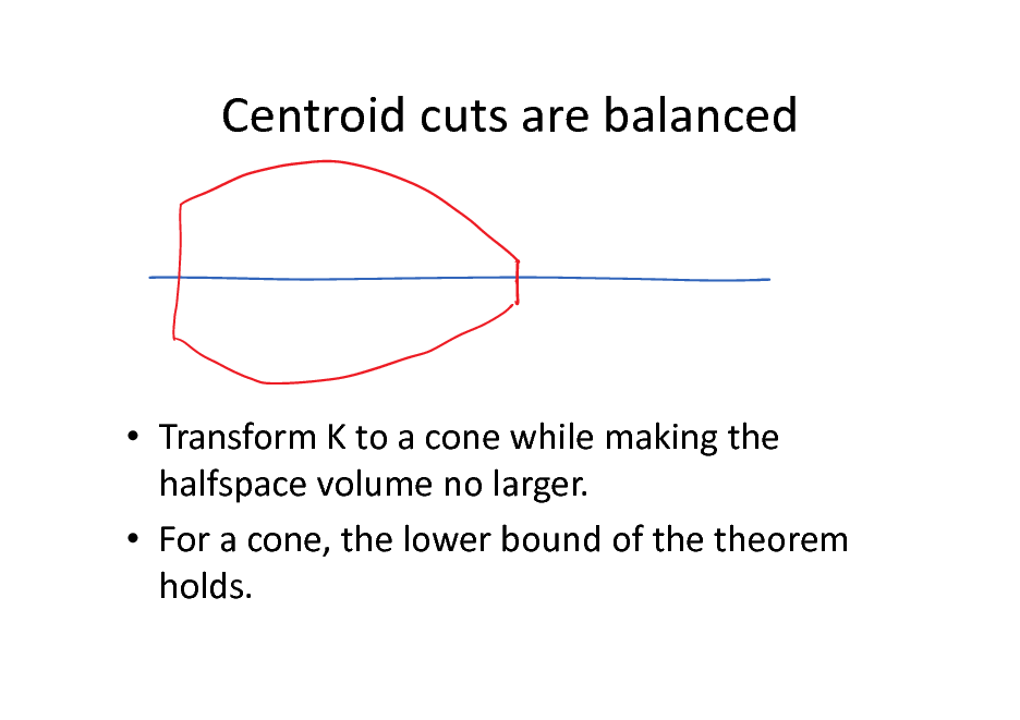
Centroid cuts are balanced
Transform K to a cone while making the halfspace volume no larger. For a cone, the lower bound of the theorem holds.
72
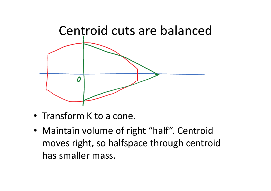
Centroid cuts are balanced
Transform K to a cone. Maintain volume of right half. Centroid moves right, so halfspace through centroid has smaller mass.
73
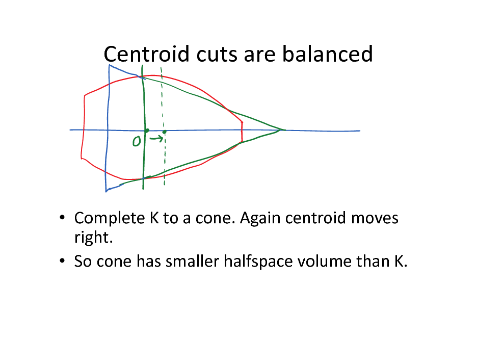
Centroid cuts are balanced
Complete K to a cone. Again centroid moves right. So cone has smaller halfspace volume than K.
74
Cone volume
Exercise 1. Show that for a cone, the volume of a halfspace containing its centroid can be as small as smaller. times its volume but no
75
Convex optimization via Sampling
How many iterations for the sampling-based algorithm? If we use only 1 random sample in each iteration, then the number of iterations could be exponential! Do poly(n) samples suffice?
76
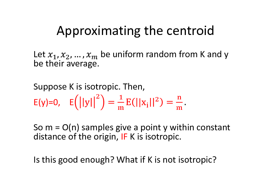
Approximating the centroid
Let be uniform random from K and y be their average. Suppose K is isotropic. Then, E(y)=0, E So m = O(n) samples give a point y within constant distance of the origin, IF K is isotropic. Is this good enough? What if K is not isotropic?
77
![Slide: Robust Grunbaum: cuts near centroid are also balanced
Lemma [BV02]. For isotropic convex body K and halfspace H containing a point within distance t of the origin,
Thm [BV02]. For any convex body K and halfspace H containing the average of m random points from K,](https://yosinski.com/mlss12/media/slides/MLSS-2012-Vempala-High-Dimensional-Sampling-Algorithms_078.png)
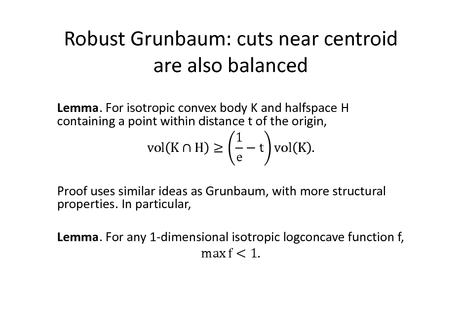
Robust Grunbaum: cuts near centroid are also balanced
Lemma [BV02]. For isotropic convex body K and halfspace H containing a point within distance t of the origin,
Thm [BV02]. For any convex body K and halfspace H containing the average of m random points from K,
78
Robust Grunbaum: cuts near centroid are also balanced
Lemma. For isotropic convex body K and halfspace H containing a point within distance t of the origin, 1 vol K H t vol K . e Proof uses similar ideas as Grunbaum, with more structural properties. In particular, Lemma. For any 1-dimensional isotropic logconcave function f, max f < 1.
79
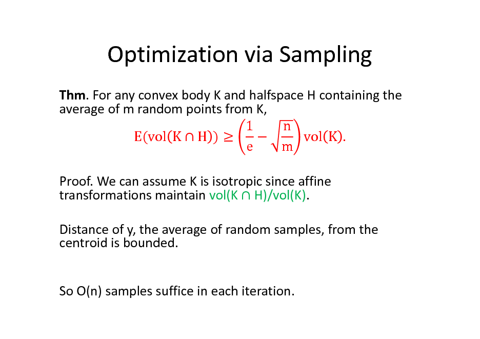
Optimization via Sampling
Thm. For any convex body K and halfspace H containing the average of m random points from K, 1 n E(vol K H ) vol K . e m Proof. We can assume K is isotropic since affine transformations maintain vol(K H)/vol(K). Distance of y, the average of random samples, from the centroid is bounded. So O(n) samples suffice in each iteration.
80
![Slide: Optimization via Sampling
Thm. [BV02] Convex feasibility can be solved using O(n log R/r) oracle calls. Ellipsoid takes , Vaidyas algorithm also takes O(n log R/r).
With sampling, one can solve convex optimization using only a membership oracle and a starting point in K. We will see this later.](https://yosinski.com/mlss12/media/slides/MLSS-2012-Vempala-High-Dimensional-Sampling-Algorithms_081.png)
Optimization via Sampling
Thm. [BV02] Convex feasibility can be solved using O(n log R/r) oracle calls. Ellipsoid takes , Vaidyas algorithm also takes O(n log R/r).
With sampling, one can solve convex optimization using only a membership oracle and a starting point in K. We will see this later.
81
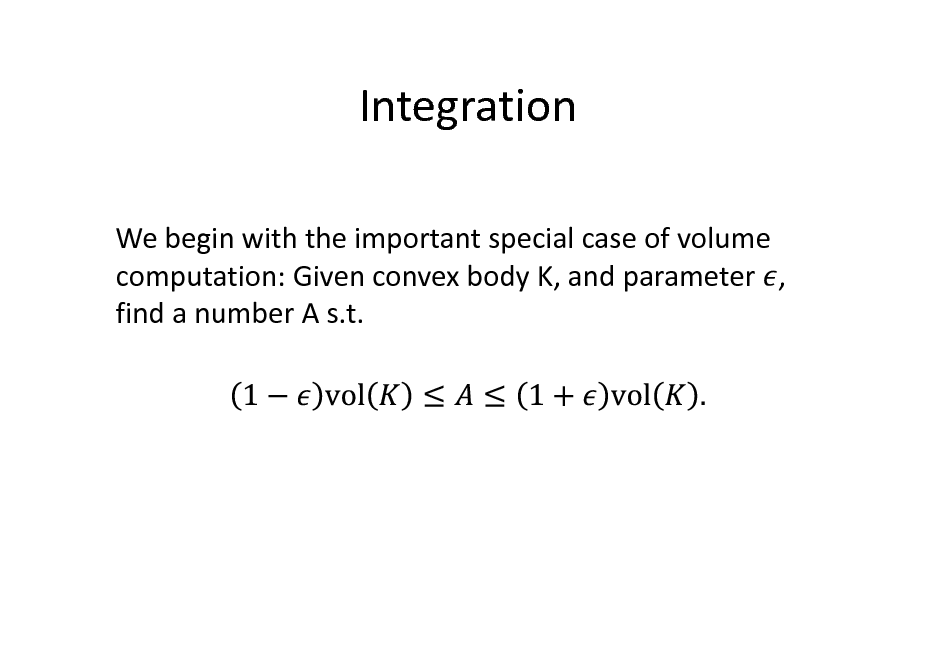
Integration
We begin with the important special case of volume computation: Given convex body K, and parameter , find a number A s.t.
82
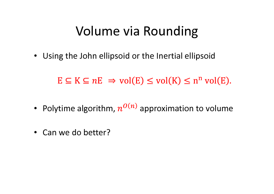
Volume via Rounding
Using the John ellipsoid or the Inertial ellipsoid
Polytime algorithm, Can we do better?
approximation to volume
83
![Slide: Complexity of Volume Estimation
Thm [E86, BF87]. For any deterministic algorithm that membership calls to the oracle for a uses at most convex body K and computes two numbers A and B , there is some convex body such that for which the ratio B/A is at least
where c is an absolute constant.](https://yosinski.com/mlss12/media/slides/MLSS-2012-Vempala-High-Dimensional-Sampling-Algorithms_084.png)
Complexity of Volume Estimation
Thm [E86, BF87]. For any deterministic algorithm that membership calls to the oracle for a uses at most convex body K and computes two numbers A and B , there is some convex body such that for which the ratio B/A is at least
where c is an absolute constant.
84
![Slide: Complexity of Volume Estimation
Thm [BF]. For deterministic algorithms: # oracle calls approximation factor
Thm [DV12]. Matching upper bound of in time](https://yosinski.com/mlss12/media/slides/MLSS-2012-Vempala-High-Dimensional-Sampling-Algorithms_085.png)
Complexity of Volume Estimation
Thm [BF]. For deterministic algorithms: # oracle calls approximation factor
Thm [DV12]. Matching upper bound of in time
85
![Slide: Volume computation
[DFK89]. Polynomial-time randomized algorithm that estimates volume with probability at least in time poly(n, ).](https://yosinski.com/mlss12/media/slides/MLSS-2012-Vempala-High-Dimensional-Sampling-Algorithms_086.png)
Volume computation
[DFK89]. Polynomial-time randomized algorithm that estimates volume with probability at least in time poly(n, ).
86
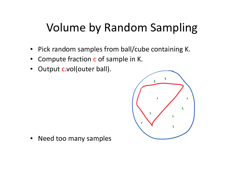
Volume by Random Sampling
Pick random samples from ball/cube containing K. Compute fraction c of sample in K. Output c.vol(outer ball).
Need too many samples
87
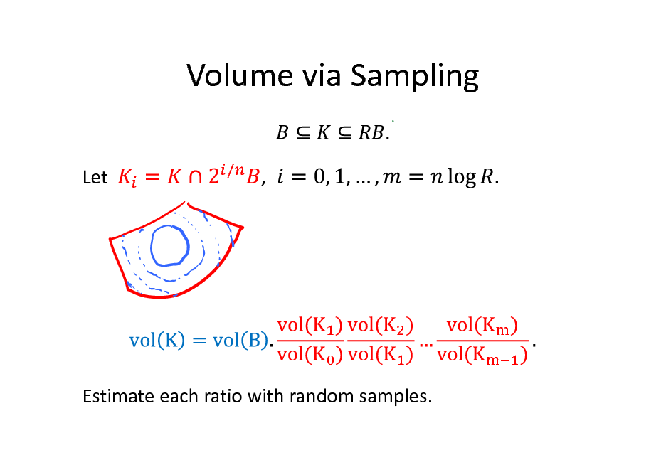
Volume via Sampling
Let
/
Estimate each ratio with random samples.
88
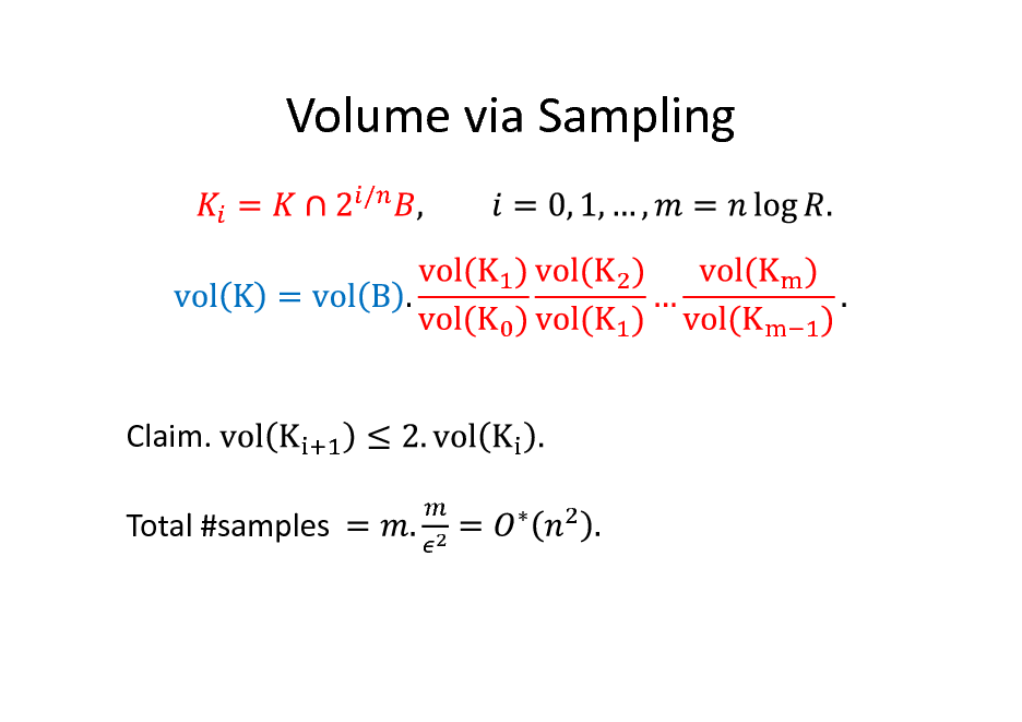
Volume via Sampling
/
Claim. Total #samples
89
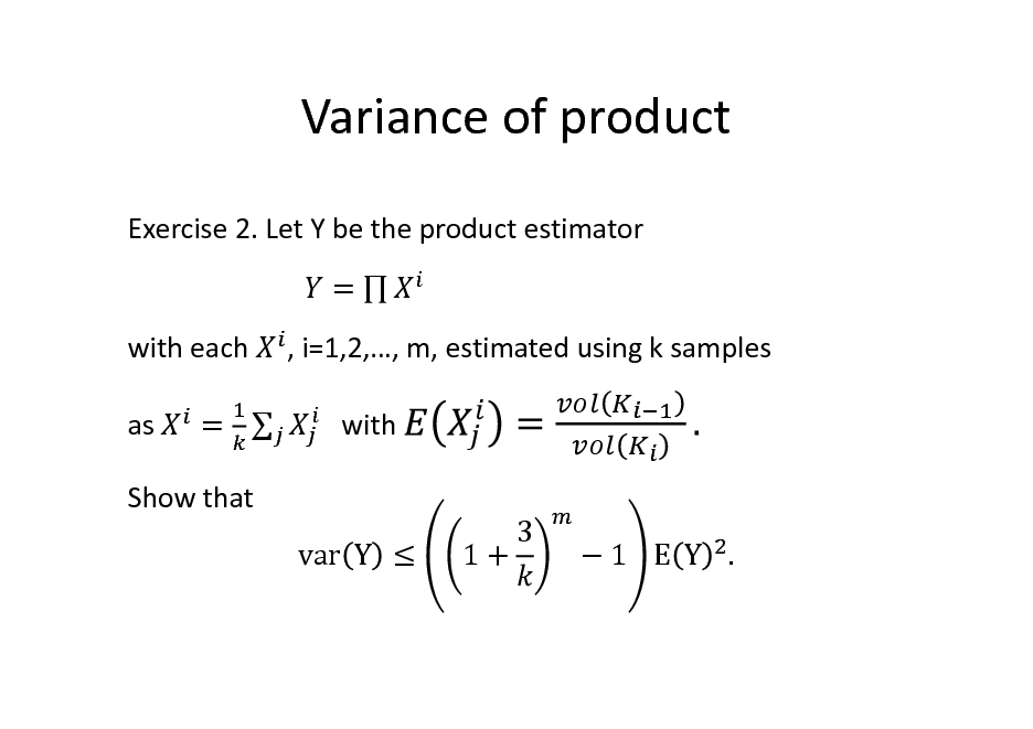
Variance of product
Exercise 2. Let Y be the product estimator = with each as = , i=1,2,, m, estimated using k samples with 3
Show that var Y 1+
1 E Y .
90
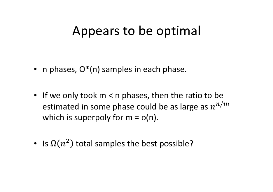
Appears to be optimal
n phases, O*(n) samples in each phase. If we only took m < n phases, then the ratio to be estimated in some phase could be as large as / which is superpoly for m = o(n). Is total samples the best possible?
91
![Slide: Simulated Annealing [Kalai-V.04,Lovasz-V.03]
To estimate consider a sequence
, ,
with Then,
,,
=
being easy, e.g., constant function over ball.
Each ratio can be estimated by sampling:
1. 2. Sample X with density proportional to Compute
=
=
.
=
.](https://yosinski.com/mlss12/media/slides/MLSS-2012-Vempala-High-Dimensional-Sampling-Algorithms_092.png)
Simulated Annealing [Kalai-V.04,Lovasz-V.03]
To estimate consider a sequence
, ,
with Then,
,,
=
being easy, e.g., constant function over ball.
Each ratio can be estimated by sampling:
1. 2. Sample X with density proportional to Compute
=
=
.
=
.
92
![Slide: A tight reduction [LV03]
Define:
~
log(2 / )](https://yosinski.com/mlss12/media/slides/MLSS-2012-Vempala-High-Dimensional-Sampling-Algorithms_093.png)
A tight reduction [LV03]
Define:
~
log(2 / )
93
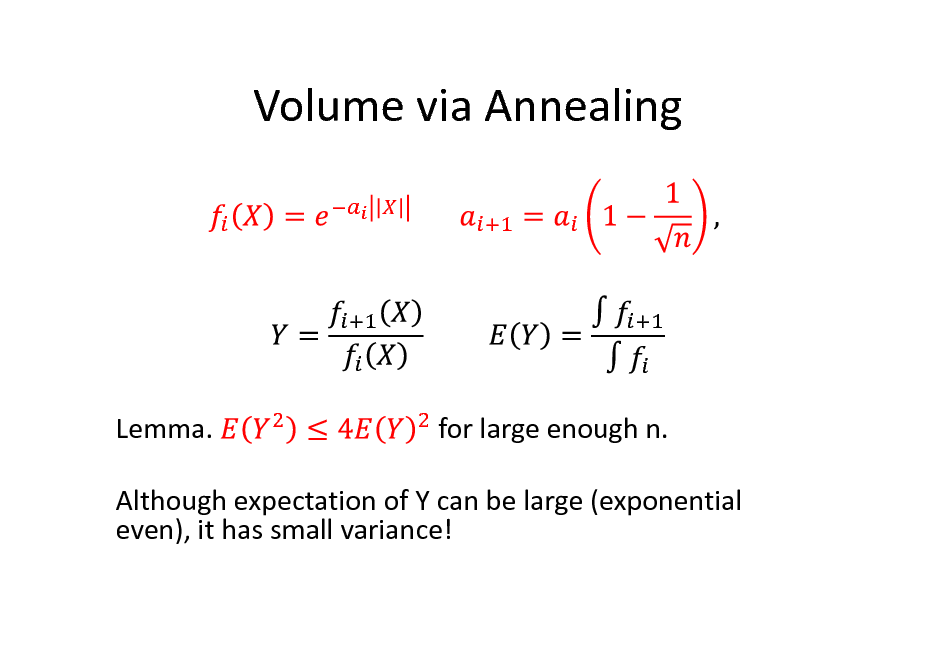
Volume via Annealing
Lemma.
for large enough n.
Although expectation of Y can be large (exponential even), it has small variance!
94
![Slide: Proof via logconcavity
Exercise 2. For a logconcave function let Show that for . is a logconcave function. ,
[Hint: Define
.]](https://yosinski.com/mlss12/media/slides/MLSS-2012-Vempala-High-Dimensional-Sampling-Algorithms_095.png)
Proof via logconcavity
Exercise 2. For a logconcave function let Show that for . is a logconcave function. ,
[Hint: Define
.]
95
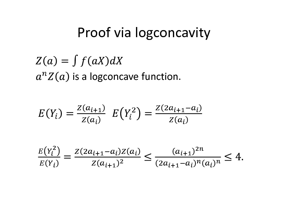
Proof via logconcavity
is a logconcave function.
96
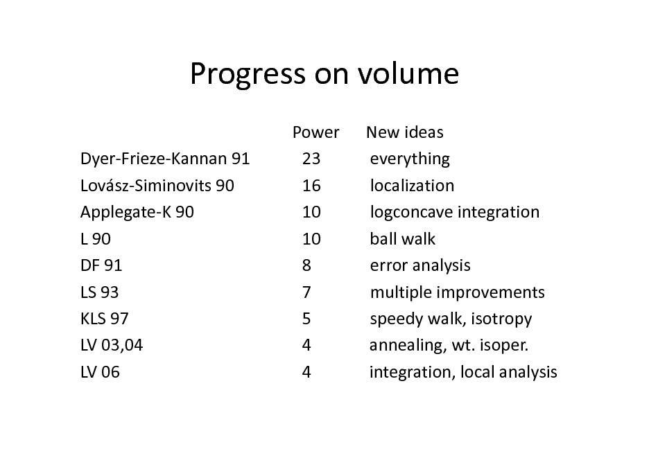
Progress on volume
Dyer-Frieze-Kannan 91 Lovsz-Siminovits 90 Applegate-K 90 L 90 DF 91 LS 93 KLS 97 LV 03,04 LV 06 Power 23 16 10 10 8 7 5 4 4 New ideas everything localization logconcave integration ball walk error analysis multiple improvements speedy walk, isotropy annealing, wt. isoper. integration, local analysis
97
![Slide: Optimization via Annealing
We can minimize quasiconvex function f over convex set S given only by a membership oracle and a starting point in S. [KV04, LV06]. Almost the same algorithm, in reverse: to find max f, define M. sequence of functions starting at nearly uniform and getting more and more concentrated points of near-optimal objective value.](https://yosinski.com/mlss12/media/slides/MLSS-2012-Vempala-High-Dimensional-Sampling-Algorithms_098.png)
Optimization via Annealing
We can minimize quasiconvex function f over convex set S given only by a membership oracle and a starting point in S. [KV04, LV06]. Almost the same algorithm, in reverse: to find max f, define M. sequence of functions starting at nearly uniform and getting more and more concentrated points of near-optimal objective value.
98

Lecture 3: Sampling Algorithms
Sampling by random walks Conductance Grid walk, Ball walk, Hit-and-run Isoperimetric inequalities Rapid mixing
99
High-Dimensional Sampling Algorithms
Santosh Vempala
Algorithms and Randomness Center Georgia Tech
100
Sampling
Generate a uniform random point from a set S or with density proportional to function f. Numerous applications in diverse areas: statistics, networking, biology, computer vision, privacy, operations research etc. This course: mathematical and algorithmic foundations of sampling and its applications.
101
Structure
Q. What geometric structure makes algorithmic problems computationally tractable?
(i.e., solvable with polynomial complexity)
Convexity often suffices. Is convexity the frontier of polynomial-time solvability? Appears to be in many cases of interest
102

Convexity
(Indicator functions of) Convex sets: , , 0,1 , , + 1 Concave functions: + 1 Logconcave functions: + 1 Quasiconcave functions: + 1 min Star-shaped sets: . . , + 1 ,
+ 1
103
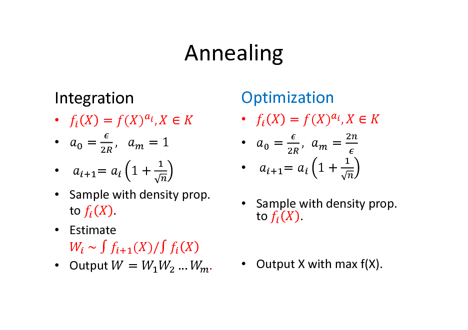
Annealing
Integration
= = = ( ) , , =1 1+
Optimization
= = = ( ) , , = 1+
Sample with density prop. . to Estimate ~ ( )/ Output = .
Sample with density prop. to .
Output X with max f(X).
104
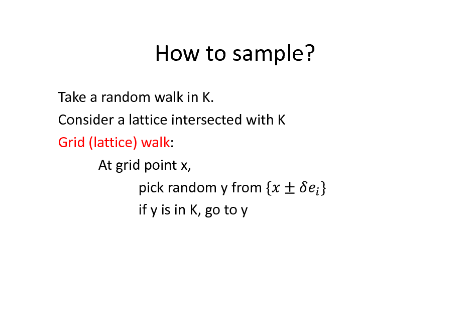
How to sample?
Take a random walk in K. Consider a lattice intersected with K Grid (lattice) walk: At grid point x, pick random y from if y is in K, go to y
105
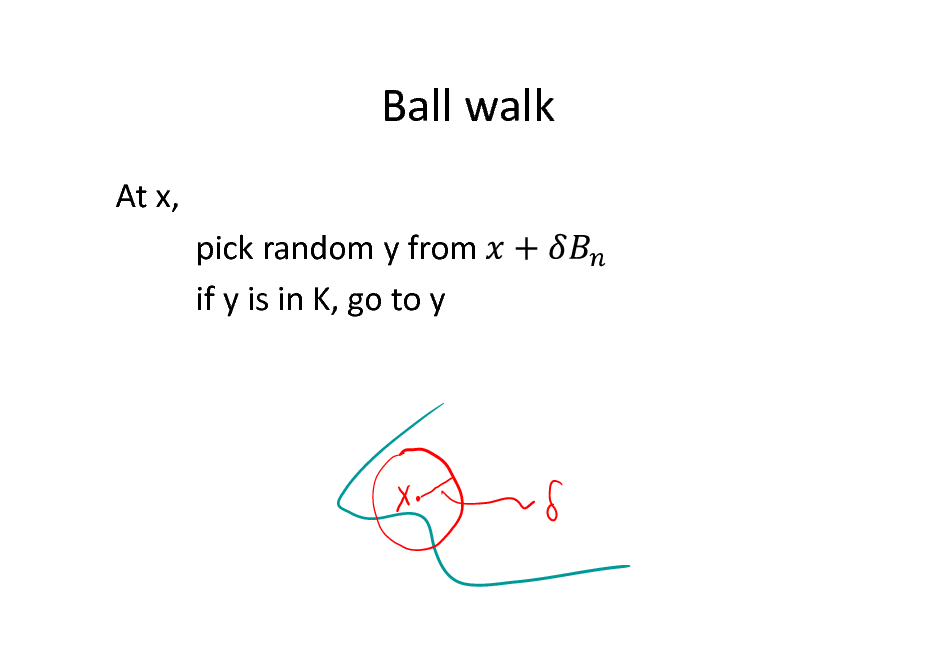
Ball walk
At x, pick random y from if y is in K, go to y
106
![Slide: Hit-and-run
[Boneh, Smith] At x, -pick a random chord L through x -go to a uniform random point y on L](https://yosinski.com/mlss12/media/slides/MLSS-2012-Vempala-High-Dimensional-Sampling-Algorithms_107.png)
Hit-and-run
[Boneh, Smith] At x, -pick a random chord L through x -go to a uniform random point y on L
107

Markov chains
State space K, set of measurable subsets that form a -algebra, i.e., closed under finite unions and intersections associated with A next step distribution each point u in the state space. A starting point. s.t.
108
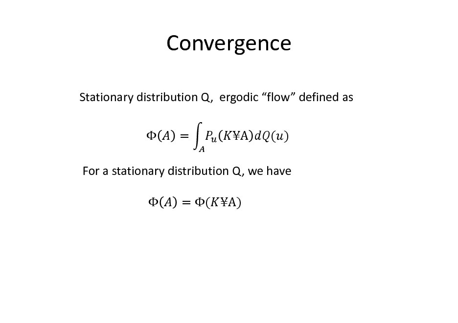
Convergence
Stationary distribution Q, ergodic flow defined as = A ( )
For a stationary distribution Q, we have = ( A)
109
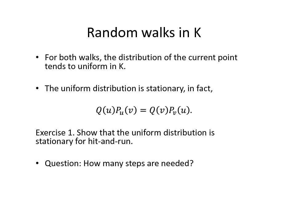
Random walks in K
For both walks, the distribution of the current point tends to uniform in K. The uniform distribution is stationary, in fact,
Exercise 1. Show that the uniform distribution is stationary for hit-and-run. Question: How many steps are needed?
110
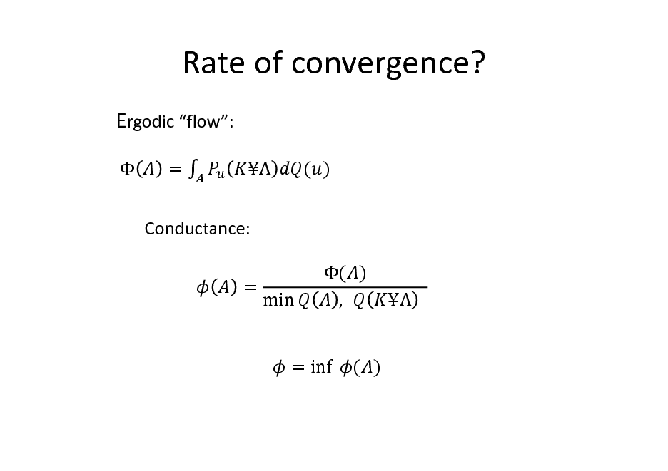
Rate of convergence?
Ergodic flow:
= A ( )
Conductance: = ( ) ,
min
A
= inf ( )
111
![Slide: Conductance
Mixing rate cannot be faster than 1/ Since it takes this many steps to even escape from some subsets. Does give an upper bound? Yes, for discrete Markov chains
Thm. [Jerrum-Sinclair]
Where is the second eigenvalue of the transition matrix.
Thus, mixing rate =](https://yosinski.com/mlss12/media/slides/MLSS-2012-Vempala-High-Dimensional-Sampling-Algorithms_112.png)
Conductance
Mixing rate cannot be faster than 1/ Since it takes this many steps to even escape from some subsets. Does give an upper bound? Yes, for discrete Markov chains
Thm. [Jerrum-Sinclair]
Where is the second eigenvalue of the transition matrix.
Thus, mixing rate =
112
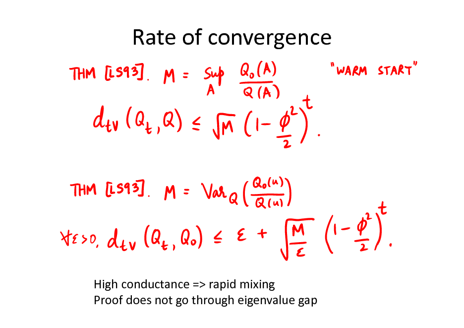
Rate of convergence
High conductance => rapid mixing Proof does not go through eigenvalue gap
113
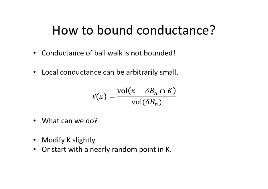
How to bound conductance?
Conductance of ball walk is not bounded! Local conductance can be arbitrarily small. What can we do? Modify K slightly Or start with a nearly random point in K. = vol + vol( )
114
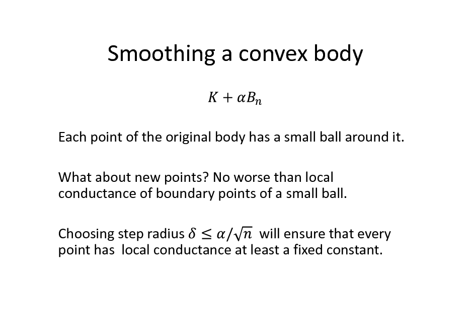
Smoothing a convex body
Each point of the original body has a small ball around it. What about new points? No worse than local conductance of boundary points of a small ball. Choosing step radius will ensure that every point has local conductance at least a fixed constant.
115
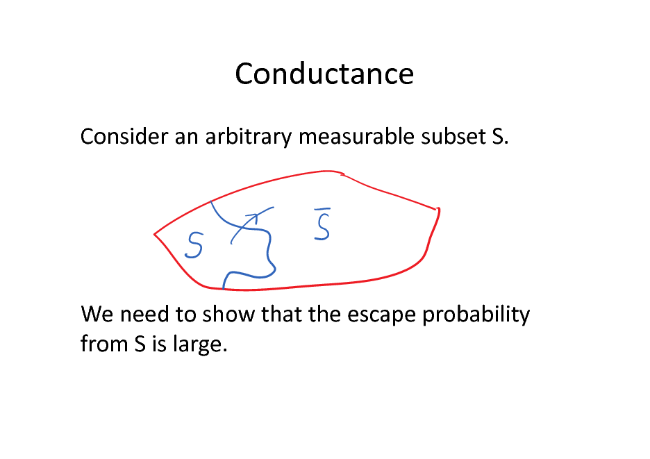
Conductance
Consider an arbitrary measurable subset S.
We need to show that the escape probability from S is large.
116
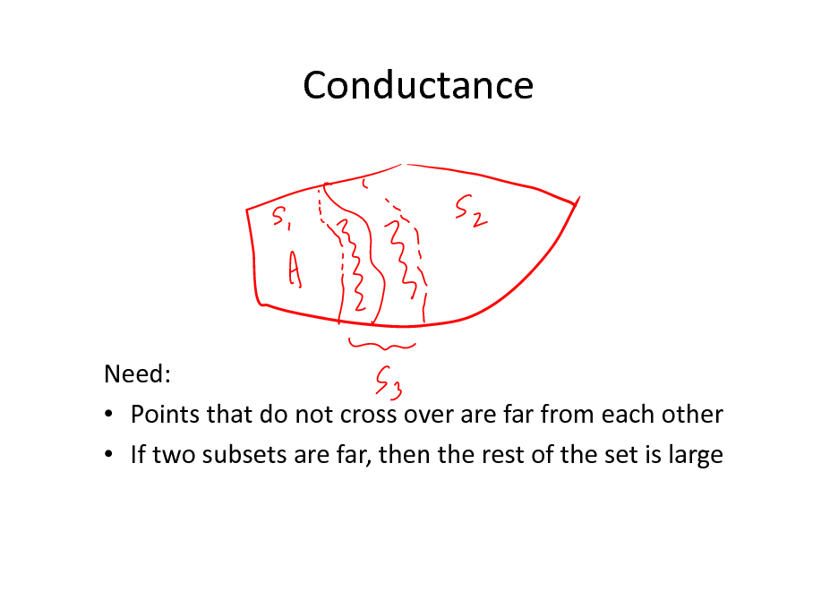
Conductance
Need: Points that do not cross over are far from each other If two subsets are far, then the rest of the set is large
117
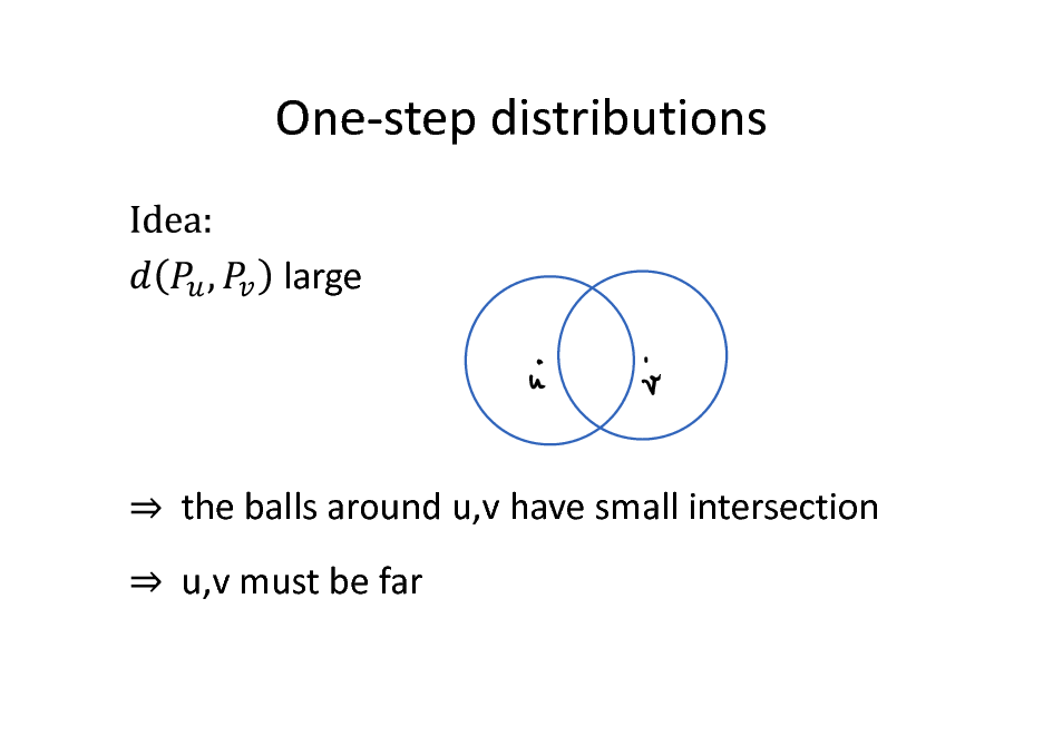
One-step distributions
large
the balls around u,v have small intersection u,v must be far
118
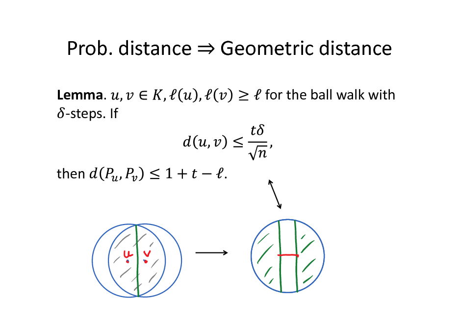
Prob. distance
Lemma. -steps. If
Geometric distance
for the ball walk with
then
.
119
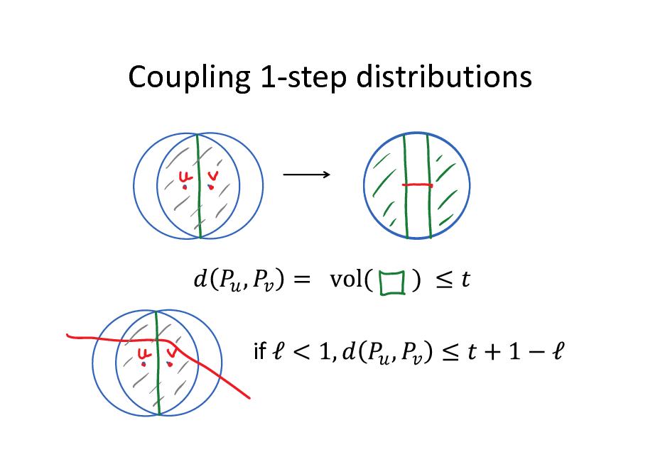
Coupling 1-step distributions
if
120
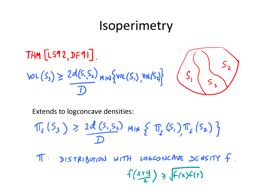
Isoperimetry
Extends to logconcave densities:
121
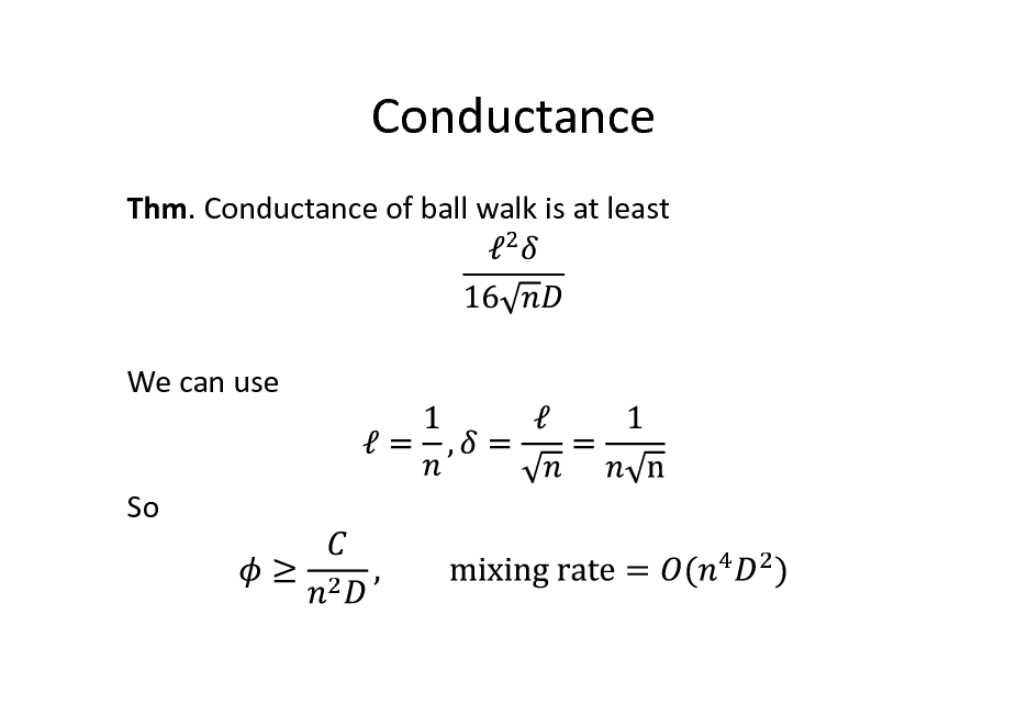
Conductance
Thm. Conductance of ball walk is at least
We can use
So
122
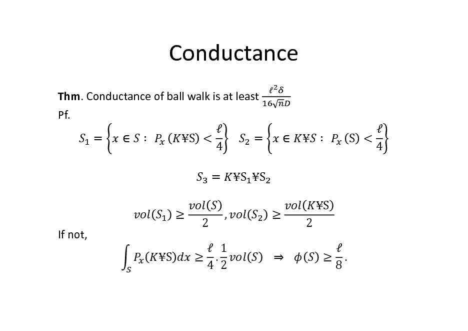
Conductance
Thm. Conductance of ball walk is at least Pf. = S < = 4 = If not, S , S S S 2 . 8
S < 4
2
1 . 4 2
123
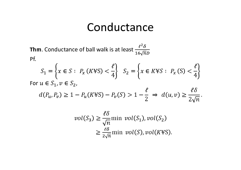
Conductance
Thm. Conductance of ball walk is at least Pf. = S < = 4 For , , , 1 S
S < 4 , 2 .
> 1 2 , ,
min min
S .
124
Conductance
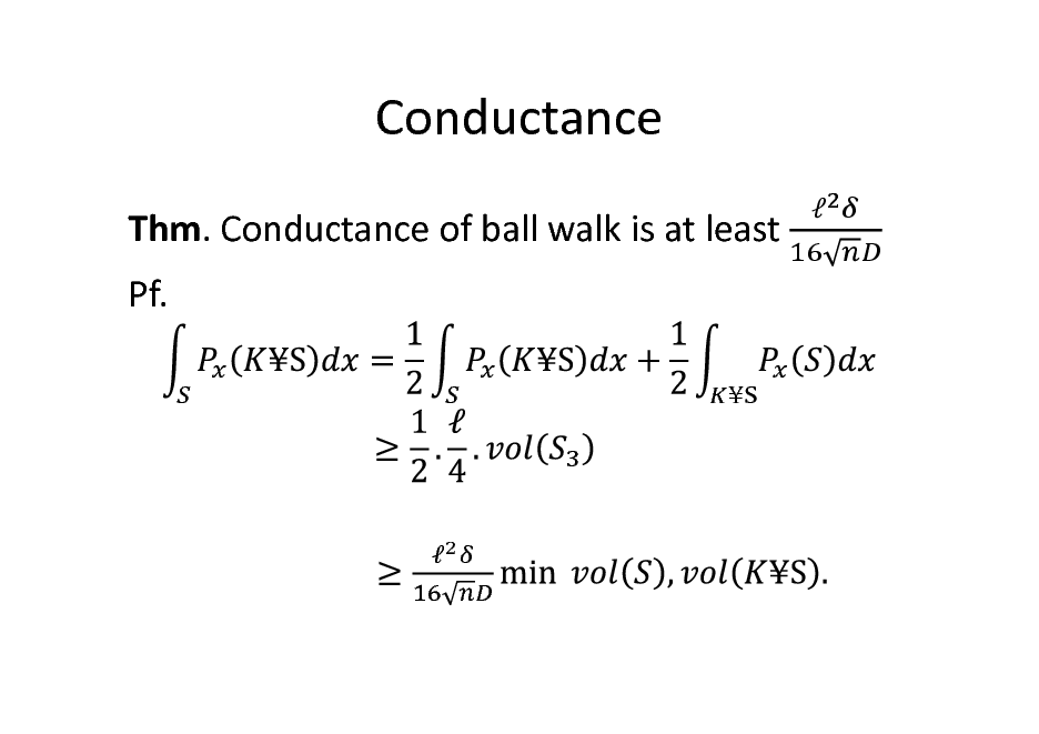
Thm. Conductance of ball walk is at least Pf.
125
KLS hyperplane conjecture
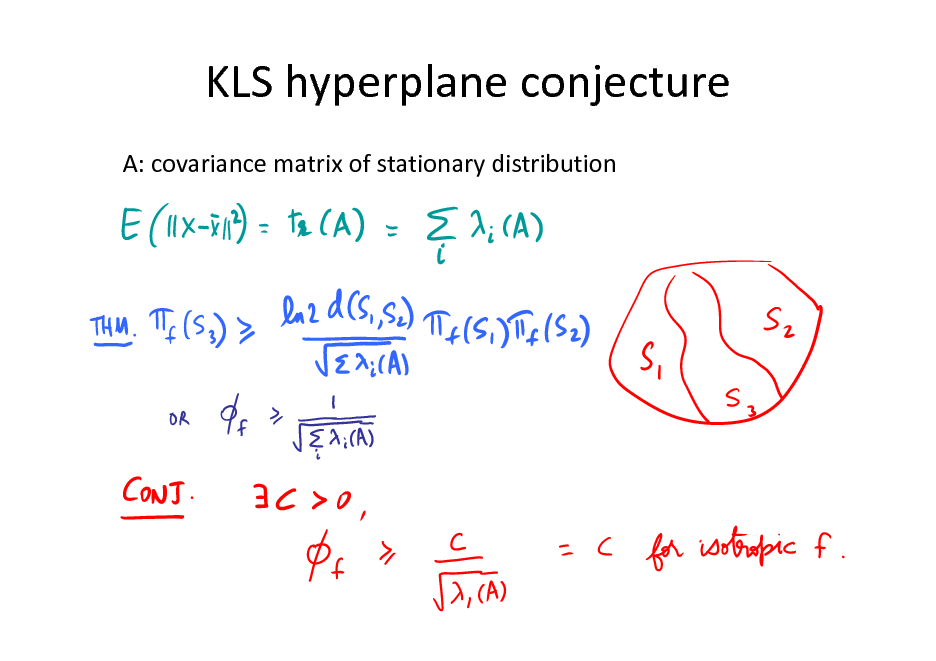
A: covariance matrix of stationary distribution
126
![Slide: Thin shell conjecture
Theorem [Bobkov].
Conj. (Thin shell) Alternatively: Current best bound [Guedon-E. Milman]: n1/3](https://yosinski.com/mlss12/media/slides/MLSS-2012-Vempala-High-Dimensional-Sampling-Algorithms_127.png)
Thin shell conjecture
Theorem [Bobkov].
Conj. (Thin shell) Alternatively: Current best bound [Guedon-E. Milman]: n1/3
127
![Slide: KLS-Slicing-Thin-shell
known conj thin shell slicing KLS
Moreover, KLS implies the others [Ball] and thinshell implies slicing [Eldan-Klartag10].](https://yosinski.com/mlss12/media/slides/MLSS-2012-Vempala-High-Dimensional-Sampling-Algorithms_128.png)
KLS-Slicing-Thin-shell
known conj thin shell slicing KLS
Moreover, KLS implies the others [Ball] and thinshell implies slicing [Eldan-Klartag10].
128
![Slide: Convergence
Thm. [LS93, KLS97] If S is convex, then the ball walk with an M-warm start reaches an (independent) nearly random point in poly(n, D, M) steps. Strictly speaking, this is not rapid mixing! How to get the first random point? Better dependence on diameter D?](https://yosinski.com/mlss12/media/slides/MLSS-2012-Vempala-High-Dimensional-Sampling-Algorithms_129.png)
Convergence
Thm. [LS93, KLS97] If S is convex, then the ball walk with an M-warm start reaches an (independent) nearly random point in poly(n, D, M) steps. Strictly speaking, this is not rapid mixing! How to get the first random point? Better dependence on diameter D?
129
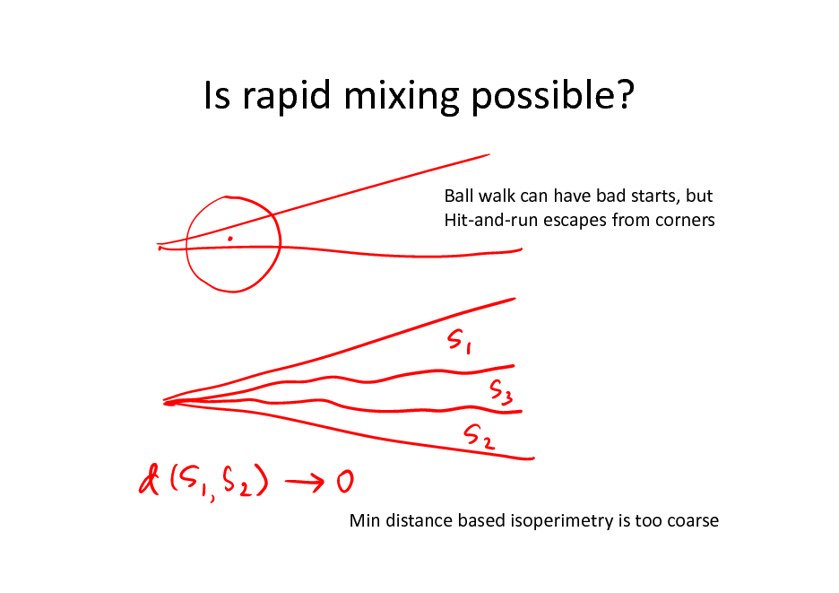
Is rapid mixing possible?
Ball walk can have bad starts, but Hit-and-run escapes from corners
Min distance based isoperimetry is too coarse
130
![Slide: Average distance isoperimetry
How to average distance?
Theorem.[LV04; Dieker-V.12]](https://yosinski.com/mlss12/media/slides/MLSS-2012-Vempala-High-Dimensional-Sampling-Algorithms_131.png)
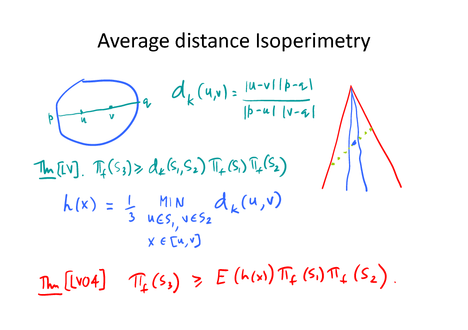
Average distance isoperimetry
How to average distance?
Theorem.[LV04; Dieker-V.12]
131
Average distance Isoperimetry
132
![Slide: Hit-and-run
Thm [LV04]. Hit-and-run mixes in polynomial time from any starting point inside a convex body. Conductance = Gives
sampling algorithm](https://yosinski.com/mlss12/media/slides/MLSS-2012-Vempala-High-Dimensional-Sampling-Algorithms_133.png)
Hit-and-run
Thm [LV04]. Hit-and-run mixes in polynomial time from any starting point inside a convex body. Conductance = Gives
sampling algorithm
133
Multi-point random walks
Maintain m points For each point X,
Pick a random combination of the m points Use this to update X
Stationary distribution: m uniform random points!
134
Sampling
Q1. Is starting at a nice point faster? E.g., does ball walk mix rapidly starting at a single point, e.g., the centroid? Q2. How to check convergence to stationarity on the fly? Does it suffice to check that the measures of all halfspaces have converged?
(Note: poly(n) sample can estimate all halfspace measures approximately)
135
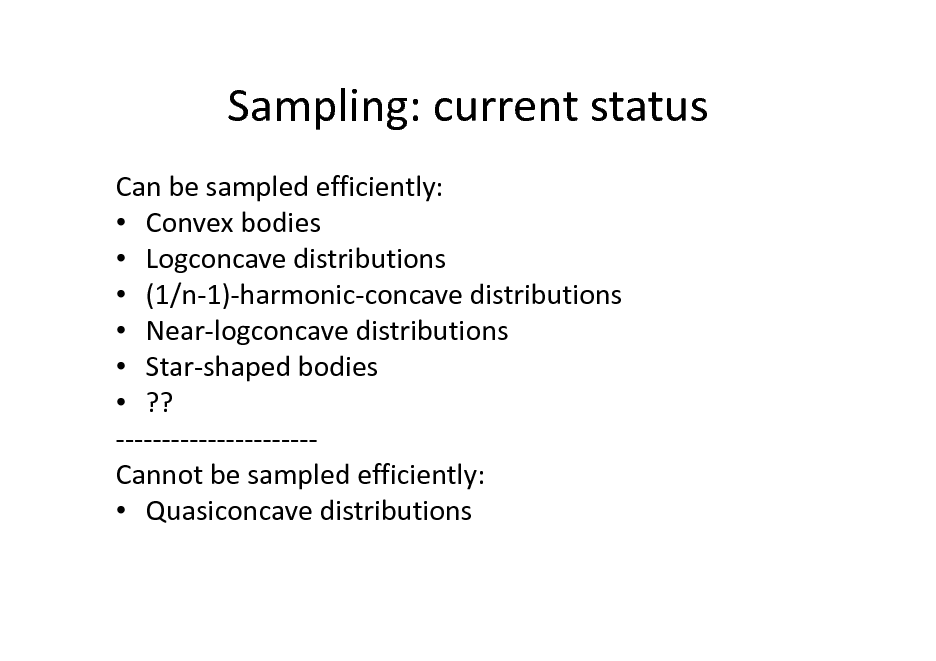
Sampling: current status
Can be sampled efficiently: Convex bodies Logconcave distributions (1/n-1)-harmonic-concave distributions Near-logconcave distributions Star-shaped bodies ?? ---------------------Cannot be sampled efficiently: Quasiconcave distributions
136
High-dimensional sampling algorithms
Sampling manifolds Random reflections Deterministic sampling? Other applications
137