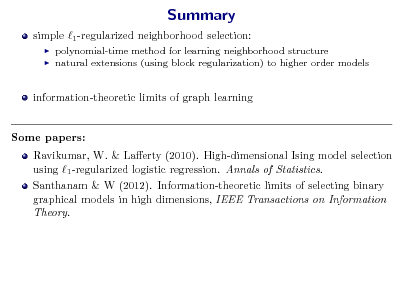
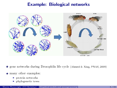
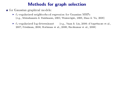
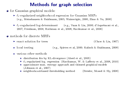
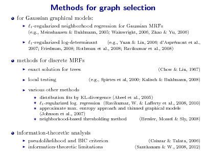
Methods for graph selection
for Gaussian graphical models:
1 -regularized neighborhood regression for Gaussian MRFs
(e.g., Meinshausen & Buhlmann, 2005; Wainwright, 2006, Zhao & Yu, 2006)
1 -regularized log-determinant
(e.g., Yuan & Lin, 2006; dAsprmont et al., e 2007; Friedman, 2008; Rothman et al., 2008; Ravikumar et al., 2008)
methods for discrete MRFs
exact solution for trees local testing various other methods
(Chow & Liu, 1967) (e.g., Spirtes et al, 2000; Kalisch & Buhlmann, 2008)
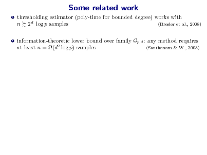
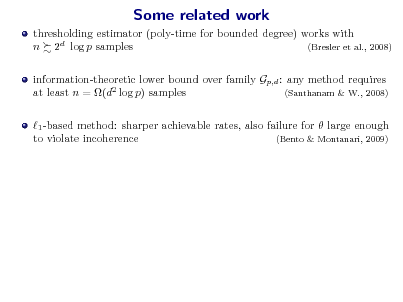
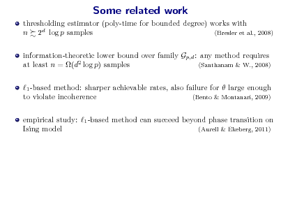
distribution ts by KL-divergence (Abeel et al., 2005) 1 -regularized log. regression (Ravikumar, W. & Laerty et al., 2008, 2010) approximate max. entropy approach and thinned graphical models (Johnson et al., 2007) neighborhood-based thresholding method (Bresler, Mossel & Sly, 2008)
information-theoretic analysis
pseudolikelihood and BIC criterion information-theoretic limitations
(Csiszar & Talata, 2006) (Santhanam & W., 2008, 2012)


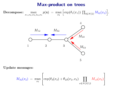
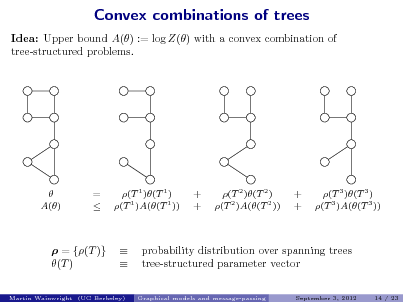
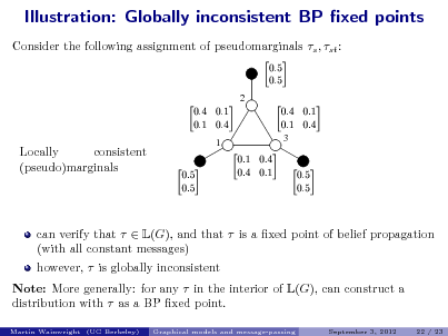
![Slide: Goal: Compute most probable conguration (MAP estimate) on a tree: exp(s (xs ) exp(st (xs , xt )) . x = arg max xX N
sV (s,t)E
1. Max-product message-passing on trees
M12
M32
1
2
3
x1 ,x2 ,x3
max p(x) = max exp(2 (x2 ))
x2 t1,3
max exp[t (xt ) + 2t (x2 , xt )]
xt
Max-product strategy: Divide and conquer: break global maximization into simpler sub-problems. (Lauritzen & Spiegelhalter, 1988)](https://yosinski.com/mlss12/media/slides/MLSS-2012-Wainwright-Graphical-Models-and-Message-Passing_012.png)


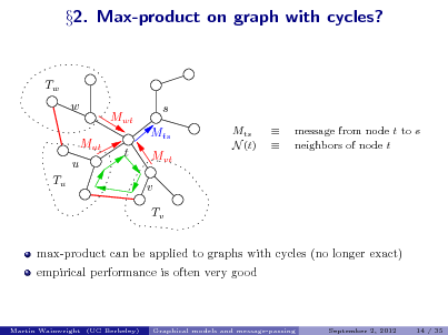


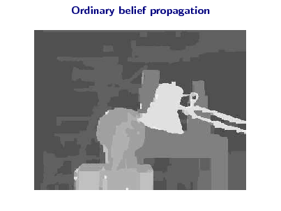
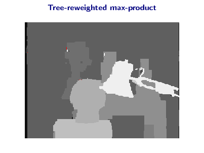
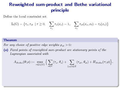
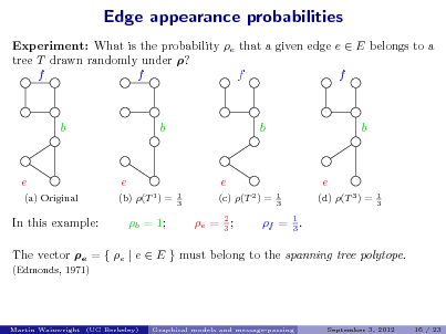
![Slide: Tree-reweighted max-product algorithms
(Wainwright, Jaakkola & Willsky, 2002)
Message update from node t to node s:
reweighted messages st (xs , x ) t + t (x ) exp t st reweighted edge Mvt (xt )
vN (t)\s vt
Mts (xs )
max
xt Xt
Mst (xt )
(1ts )
.
opposite message
Properties: 1. Modied updates remain distributed and purely local over the graph. Messages are reweighted with st [0, 1]. 2. Key dierences: Potential on edge (s, t) is rescaled by st [0, 1]. Update involves the reverse direction edge. 3. The choice st = 1 for all edges (s, t) recovers standard update.
Martin Wainwright (UC Berkeley)
Graphical models and message-passing
September 2, 2012
20 / 35](https://yosinski.com/mlss12/media/slides/MLSS-2012-Wainwright-Graphical-Models-and-Message-Passing_023.png)
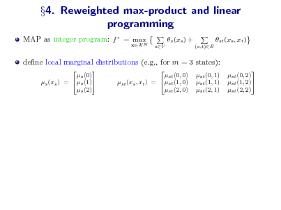
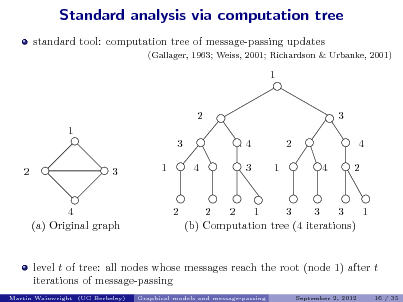
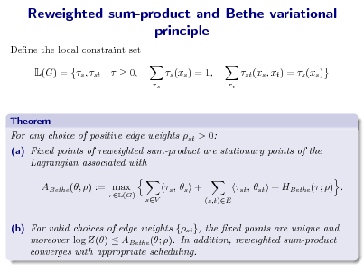
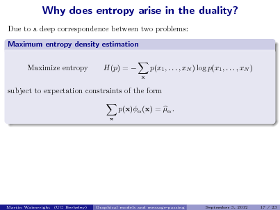
![Slide: 4. Reweighted max-product and linear programming
MAP as integer program: f = max N
xX
s (xs ) +
sV (s,t)E
st (xs , xt )
dene local marginal distributions (e.g., for m = 3 states):
s (0) s (1) s (xs ) = s (2) st (0, 0) st (xs , xt ) = st (1, 0) st (2, 0) st (0, 1) st (1, 1) st (2, 1) st (0, 2) st (1, 2) st (2, 2)
alternative formulation of MAP as linear program? g =
(s ,st )M(G)
max
Es [s (xs )]
sV
+
(s,t)E
Est [st (xs , xt )] s (xs )s (xs ).
xs
Local expectations:
Es [s (xs )]
:=](https://yosinski.com/mlss12/media/slides/MLSS-2012-Wainwright-Graphical-Models-and-Message-Passing_026.png)
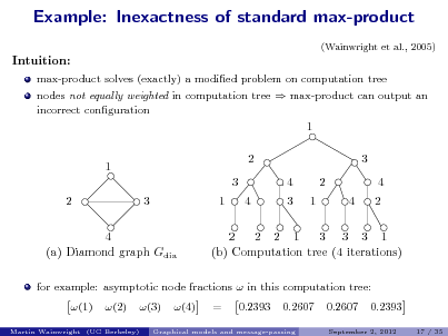
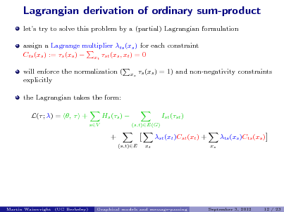
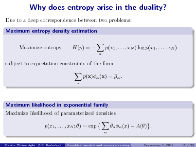
![Slide: 4. Reweighted max-product and linear programming
MAP as integer program: f = max N
xX
s (xs ) +
sV (s,t)E
st (xs , xt )
dene local marginal distributions (e.g., for m = 3 states):
s (0) s (1) s (xs ) = s (2) st (0, 0) st (xs , xt ) = st (1, 0) st (2, 0) st (0, 1) st (1, 1) st (2, 1) st (0, 2) st (1, 2) st (2, 2)
alternative formulation of MAP as linear program? g =
(s ,st )M(G)
max
Es [s (xs )]
sV
+
(s,t)E
Est [st (xs , xt )] s (xs )s (xs ).
xs
Local expectations:
Es [s (xs )]
:=
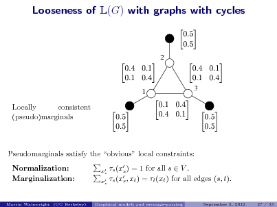
Key question: What constraints must local marginals {s , st } satisfy?](https://yosinski.com/mlss12/media/slides/MLSS-2012-Wainwright-Graphical-Models-and-Message-Passing_027.png)


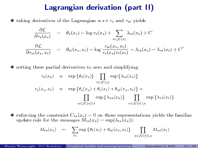
![Slide: Max-product on trees: Linear program solver
MAP problem as a simple linear program: Es [s (xs )] + f (x) = arg max M(T )
sV
Est [st (xs , xt )]
(s,t)E
.
Max-product and LP solving:
subject to in tree marginal polytope: s (xs ) = 1, M(T ) = 0, x
s
st (xs , x ) = s (xs ) t
xt
on tree-structured graphs, max-product is a dual algorithm for solving the tree LP. (Wai. & Jordan, 2003) max-product message Mts (xs ) Lagrange multiplier for enforcing the constraint x st (xs , x ) = s (xs ). t
t Martin Wainwright (UC Berkeley) Graphical models and message-passing September 2, 2012 25 / 35](https://yosinski.com/mlss12/media/slides/MLSS-2012-Wainwright-Graphical-Models-and-Message-Passing_030.png)
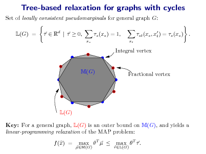
![Slide: TRW max-product and LP relaxation
First-order (tree-based) LP relaxation: f (x) max Es [s (xs )] + L(G)
sV
Est [st (xs , xt )]
(s,t)E
Results:
(Wainwright et al., 2005; Kolmogorov & Wainwright, 2005):
(a) Strong tree agreement Any TRW xed-point that satises the strong tree agreement condition species an optimal LP solution. (b) LP solving: For any binary pairwise problem, TRW max-product solves the rst-order LP relaxation. (c) Persistence for binary problems: Let S V be the subset of vertices for which there exists a single point x arg maxxs s (xs ). Then for any s optimal solution, it holds that ys = xs .
Martin Wainwright (UC Berkeley)
Graphical models and message-passing
September 2, 2012
28 / 35](https://yosinski.com/mlss12/media/slides/MLSS-2012-Wainwright-Graphical-Models-and-Message-Passing_033.png)


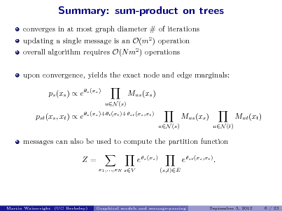
![Slide: Goal: Compute marginal distribution at node u on a tree: x = arg max exp(s (xs ) exp(st (xs , xt )) . xX N
sV (s,t)E
1. Sum-product message-passing on trees
M12
M32
1
2
3
p(x) =
x1 ,x2 ,x3 x2
exp(1 (x1 ))
t1,3 xt
exp[t (xt ) + 2t (x2 , xt )]](https://yosinski.com/mlss12/media/slides/MLSS-2012-Wainwright-Graphical-Models-and-Message-Passing_044.png)


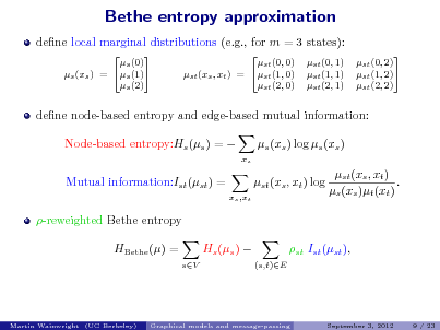
![Slide: Tree-reweighted sum-product algorithms
Message update from node t to node s:
reweighted messages st (xs , x ) t exp + t (x ) t st reweighted edge Mvt (xt )
vN (t)\s vt
Mts (xs )
x Xt t
Mst (xt )
(1ts )
.
opposite message
Properties: 1. Modied updates remain distributed and purely local over the graph. Messages are reweighted with st [0, 1]. 2. Key dierences: Potential on edge (s, t) is rescaled by st [0, 1]. Update involves the reverse direction edge. 3. The choice st = 1 for all edges (s, t) recovers standard update.
Martin Wainwright (UC Berkeley)
Graphical models and message-passing
September 3, 2012
8 / 23](https://yosinski.com/mlss12/media/slides/MLSS-2012-Wainwright-Graphical-Models-and-Message-Passing_050.png)
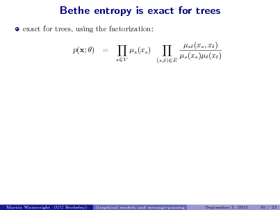


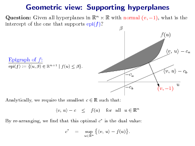
![Slide: Example: Single Bernoulli
Random variable X {0, 1} yields exponential family of the form: p(x; ) exp x Lets compute the dual A ()
R
with
A() = log 1 + exp() .
:= sup log[1 + exp()] . = exp()/[1 + exp()].
(Possible) stationary point:
A()
A()
, A ()
(a) Epigraph supported A () =
(b)
, c
Epigraph cannot be supported
We nd that:
log + (1 ) log(1 ) if [0, 1] . + otherwise. Leads to the variational representation: A() = max[0,1] A () .
Graphical models and message-passing September 3, 2012 20 / 23
Martin Wainwright (UC Berkeley)](https://yosinski.com/mlss12/media/slides/MLSS-2012-Wainwright-Graphical-Models-and-Message-Passing_067.png)


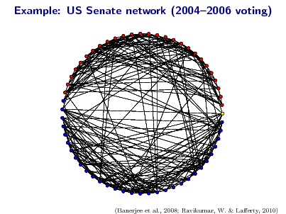
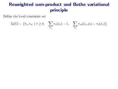
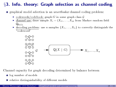
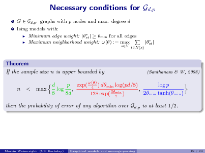
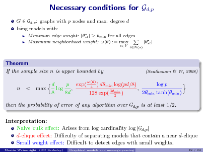
![Slide: Learning for pairwise models
drawn n samples from Q(x1 , . . . , xp ; ) = 1 exp Z() s x2 + s
sV (s,t)E
st xs xt
graph G and matrix []st = st of edge weights are unknown
Martin Wainwright (UC Berkeley)
Graphical models and message-passing
5 / 24](https://yosinski.com/mlss12/media/slides/MLSS-2012-Wainwright-Graphical-Models-and-Message-Passing_075.png)
![Slide: Learning for pairwise models
drawn n samples from Q(x1 , . . . , xp ; ) = 1 exp Z() s x2 + s
sV (s,t)E
st xs xt
graph G and matrix []st = st of edge weights are unknown data matrix:
Ising model (binary variables): Xn {0, 1}np 1 Gaussian model: Xn Rnp 1
estimator Xn 1
Martin Wainwright (UC Berkeley)
Graphical models and message-passing
5 / 24](https://yosinski.com/mlss12/media/slides/MLSS-2012-Wainwright-Graphical-Models-and-Message-Passing_076.png)
![Slide: Learning for pairwise models
drawn n samples from Q(x1 , . . . , xp ; ) = 1 exp Z() s x2 + s
sV (s,t)E
st xs xt
graph G and matrix []st = st of edge weights are unknown data matrix:
Ising model (binary variables): Xn {0, 1}np 1 Gaussian model: Xn Rnp 1
estimator Xn 1 various loss functions are possible:
graph selection: supp[] = supp[]? bounds on Kullback-Leibler divergence D(Q bounds on ||| |||op .
Graphical models and message-passing
Q )
Martin Wainwright (UC Berkeley)
5 / 24](https://yosinski.com/mlss12/media/slides/MLSS-2012-Wainwright-Graphical-Models-and-Message-Passing_077.png)

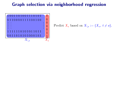
![Slide: Graph selection via neighborhood regression
1001101001110101 0110000111100100 ..... ..... 1111110101011011 0011010101000101 ..... 1 0 0 0 0 1 1
Predict Xs based on X\s := {Xs , t = s}.
X\s
1
Xs
For each node s V , compute (regularized) max. likelihood estimate: [s] := arg min p1
R
1 n
n i=1
L(; Xi, \s )
+
n
1
local log. likelihood
regularization](https://yosinski.com/mlss12/media/slides/MLSS-2012-Wainwright-Graphical-Models-and-Message-Passing_087.png)
![Slide: Graph selection via neighborhood regression
1001101001110101 0110000111100100 ..... ..... 1111110101011011 0011010101000101 ..... 1 0 0 0 0 1 1
Predict Xs based on X\s := {Xs , t = s}.
X\s
1
Xs
For each node s V , compute (regularized) max. likelihood estimate: [s] := arg min p1
R
1 n
n i=1
L(; Xi, \s )
+
n
1
local log. likelihood
regularization
2
Estimate the local neighborhood N (s) as support of regression vector [s] Rp1 .](https://yosinski.com/mlss12/media/slides/MLSS-2012-Wainwright-Graphical-Models-and-Message-Passing_088.png)
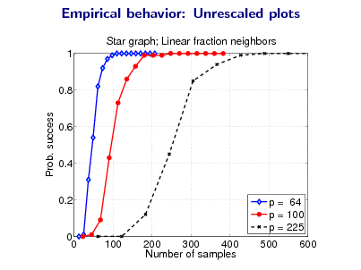
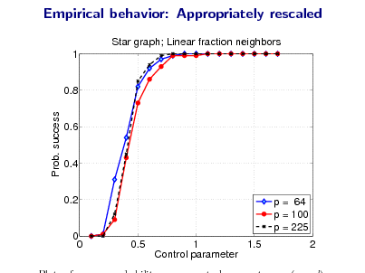
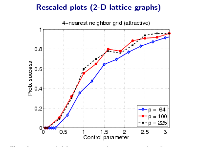
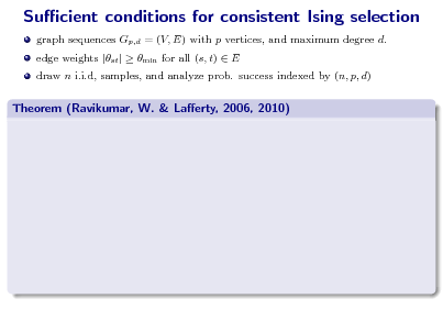
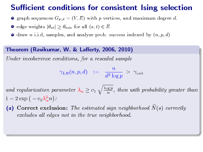
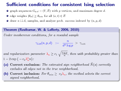
![Slide: High-dimensional analysis
classical analysis: graph size p xed, sample size n + high-dimensional analysis: allow both dimension p, sample size n, and maximum degree d to increase at arbitrary rates
take n i.i.d. samples from MRF dened by Gp,d study probability of success as a function of three parameters: Success(n, p, d) = Q[Method recovers graph Gp,d from n samples]
theory is non-asymptotic: explicit probabilities for nite (n, p, d)](https://yosinski.com/mlss12/media/slides/MLSS-2012-Wainwright-Graphical-Models-and-Message-Passing_089.png)


![Slide: Proof sketch: Main ideas for necessary conditions
based on assessing diculty of graph selection over various sub-ensembles G Gp,d choose G G u.a.r., and consider multi-way hypothesis testing problem based on the data Xn = {X1 , . . . , Xn } 1 for any graph estimator : X n G, Fanos inequality implies that Q[(Xn ) = G] 1 1 I(Xn ; G) + log 2 1 log |G|
where I(Xn ; G) is mutual information between observations Xn and 1 1 randomly chosen graph G
Martin Wainwright (UC Berkeley)
Graphical models and message-passing
21 / 24](https://yosinski.com/mlss12/media/slides/MLSS-2012-Wainwright-Graphical-Models-and-Message-Passing_112.png)
![Slide: Proof sketch: Main ideas for necessary conditions
based on assessing diculty of graph selection over various sub-ensembles G Gp,d choose G G u.a.r., and consider multi-way hypothesis testing problem based on the data Xn = {X1 , . . . , Xn } 1 for any graph estimator : X n G, Fanos inequality implies that Q[(Xn ) = G] 1 1 I(Xn ; G) + log 2 1 log |G|
where I(Xn ; G) is mutual information between observations Xn and 1 1 randomly chosen graph G remaining steps:
1 2 3
Construct dicult sub-ensembles G Gp,d Compute or lower bound the log cardinality log |G|. Upper bound the mutual information I(Xn ; G). 1
Graphical models and message-passing 21 / 24
Martin Wainwright (UC Berkeley)](https://yosinski.com/mlss12/media/slides/MLSS-2012-Wainwright-Graphical-Models-and-Message-Passing_113.png)